Simpson's paradox
Categories: recreational maths paradox
Level:

Suppose there are two surgeons, A and B. They both perform the same types of surgeries. Some of those surgeries are high-risk, and some are low-risk.
The table below shows the average success rate of both surgeons for both types of surgeries.
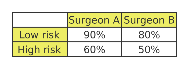
Now, two things are clear from this. First, both surgeons have a higher success rate with low-risk surgeries than with high-risk surgeries, as you might expect. And secondly, surgeon A has better results than surgeon B for both types of surgeries. It seems fair to say that surgeon A is a better surgeon than B.
But here's the strange thing. When the hospital analyses the overall success rate (the total proportion of successful operations) surgeon A has an overall success rate of 69%, whereas surgeon B has an overall success rate of 71%.
That is an example of Simpson's paradox. But what exactly is going on?
Confounding variables
The problem with the analysis above is that we have missed an important variable. We haven't taken into account the fact that the two surgeons might each take on a different proportion of low or high-risk cases.
A variable like that is called a confounding variable. They arise for various reasons:
- Simple oversight. Nobody realised that the variable existed or had any effect.
- Invalid assumption. The variable is known, but everybody assumes it doesn't make any difference. In the case above, if surgeon A performs better in both high-risk and low-risk operations, surely they should do better than surgeon B, no matter which surgeries they perform? At first glance, that seems intuitively obvious, but in fact it isn't always true. That is the apparent paradox.
- Bad actors. This paradox is sometimes used for nefarious purposes, to deliberately convince people of something that isn't true.
Analysing the surgeon example
The apparently paradoxical example above can be explained by simple arithmetic.
Let's assume that both surgeons perform 100 operations over some period of time. In that time, surgeon A performs 30 low-risk operations and 70 high-risk operations. The total number of successful operations will be given by:
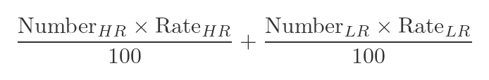
Where Number is the number of operations (either high risk, HR or low risk, LR), and Rate is the success rate. We divide by 100 because the rate is expressed as a percentage. For surgeon A, this is:
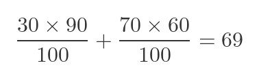
But surgeon B, being less skilled, tends to do more low risk surgeries. Over the same period, they perform 70 low-risk operations and 30 high-risk operations. Their calculation is:
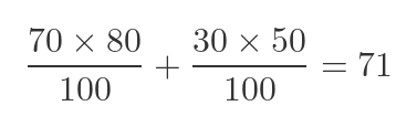
It may seem initially counterintuitive, but the maths shows what is happening. Even though surgeon B has worse results in both categories, they are doing 40 extra operations in the low-risk category (where they have an 80% success rate). Surgeon A is doing 40 extra operations in the high-risk category instead, with a success rate of 60%. That is enough to swing the result.
A famous example
In the early stages of the Covid outbreak, there were statistics floating around that claimed to prove the Covid vaccine had no benefit, and in fact that it might even be doing more harm than good.
This was completely untrue, of course. But the statistics appeared to prove it.
To illustrate this phenomenon, we will use figures from this article by the COVID-19 Actuaries Response Group. The figures are illustrative, that is to say, they are not the actual numbers, but they follow a similar pattern to the real data.
This table shows the death rates of vaccinated and unvaccinated people aged 10 to 29. Note that the death rate is the number of deaths per 100,000 population:

This assumes that around 50% of people in that age group were vaccinated, and that being vaccinated reduced the overall death rate (deaths from all causes) by 50%.
This table shows the death rates of vaccinated and unvaccinated people aged 30 to 59:

This assumes that around 90% of people were vaccinated, and again, that being vaccinated reduced the overall death rate by 50%.
It is clear from these tables that vaccinated people in both age groups had a significantly lower death rate. But what happens if we combine these two tables to find the overall death rate for everyone aged 10 to 59?
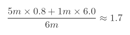
For the unvaccinated case:
- 5m people aged 10-29 had a death rate of 0.8 (per 100,000 population), so the total number of deaths was 40.
- 1m people aged 30-59 had a death rate of 6.0, so the total number of deaths was 60.
- This means that there were 100 deaths in the total population of people aged 10-59.
- Since there were a total of 6m people, this gives a death rate of about 1.7 per 100,000 people.
Here is the calculation above, expressed as a formula:
If we repeat the calculation for the vaccinated people, we get this:
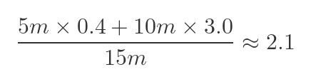
So here is a table representing the vaccinated and unvaccinated statistics for the entire group of people aged 10 to 59
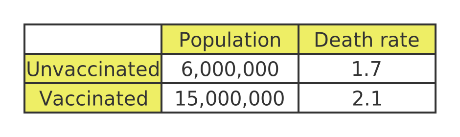
According to this, vaccinated people have a higher death rate than unvaccinated people. Even though vaccinated people aged 10-29 and vaccinated people aged 30-59 both do a lot better than their unvaccinated counterparts.
And that is technically true, but very misleading. The reason for this statistical anomaly is not that the vaccine is dangerous. It is that the vaccinated group contains a greater number of older people. Older people are a lot more likely to die of something else, unrelated to Covid or the vaccine.
Summary
When aggregating data, it is important to be aware of Simpson's paradox and the possibility that confounding variables might exist, because they can lead to misleading conclusions if not handled carefully.
Related articles
Join the GraphicMaths Newsletter
Sign up using this form to receive an email when new content is added to the graphpicmaths or pythoninformer websites:
Popular tags
adder adjacency matrix alu and gate angle answers area argand diagram binary maths cardioid cartesian equation chain rule chord circle cofactor combinations complex modulus complex numbers complex polygon complex power complex root cosh cosine cosine rule countable cpu cube decagon demorgans law derivative determinant diagonal directrix dodecagon e eigenvalue eigenvector ellipse equilateral triangle erf function euclid euler eulers formula eulers identity exercises exponent exponential exterior angle first principles flip-flop focus gabriels horn galileo gamma function gaussian distribution gradient graph hendecagon heptagon heron hexagon hilbert horizontal hyperbola hyperbolic function hyperbolic functions infinity integration integration by parts integration by substitution interior angle inverse function inverse hyperbolic function inverse matrix irrational irrational number irregular polygon isomorphic graph isosceles trapezium isosceles triangle kite koch curve l system lhopitals rule limit line integral locus logarithm maclaurin series major axis matrix matrix algebra mean minor axis n choose r nand gate net newton raphson method nonagon nor gate normal normal distribution not gate octagon or gate parabola parallelogram parametric equation pentagon perimeter permutation matrix permutations pi pi function polar coordinates polynomial power probability probability distribution product rule proof pythagoras proof quadrilateral questions quotient rule radians radius rectangle regular polygon rhombus root sech segment set set-reset flip-flop simpsons rule sine sine rule sinh slope sloping lines solving equations solving triangles square square root squeeze theorem standard curves standard deviation star polygon statistics straight line graphs surface of revolution symmetry tangent tanh transformation transformations translation trapezium triangle turtle graphics uncountable variance vertical volume volume of revolution xnor gate xor gate