Tangents and normals in polar coordinates

Polar coordinates define points in space in terms of the distance r between the point and the origin, and the angle θ that the point makes with the x-axis. Functions in polar coordinates are typically defined by specifying r as a function of θ. For example, this equation defines a cardioid curve:

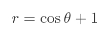
Here is a plot of the function.

Although we have defined this function in terms of r and θ, it is still a curve like any other, so we can draw a tangent to it. The red line above shows one possible tangent to the curve. But how do we find the slope of the tangent?

Finding the tangent of a polar curve

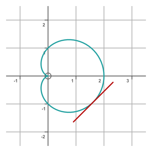
In Cartesian coordinates, the slope of a straight line is given by Δy/Δx, where Δx is the change in x and Δy is the corresponding change in y. If we draw a tangent to a curve at a point, we can find the slope of the curve at that point using Δy/Δx.

We can find the tangent to the polar curve in exactly the same way, as shown here:

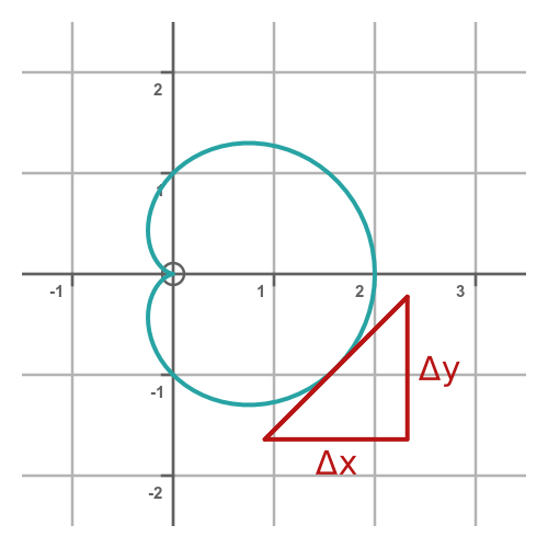
The only difference for the polar case is that the function is expressed in terms of r, θ rather than x, y, so we have to do a little bit of extra work.

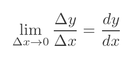
In Cartesian coordinates, we often use differentiation to find the slope of the curve at a point. In effect, we let Δy and Δx get smaller and smaller. As they tend to zero, their ratio tends towards the slope of the curve at that point. We can say that:

We use exactly that same method for polar functions, but again we need to do a bit of extra work because the formula is not expressed in terms of x and y.

Polar tangent formula

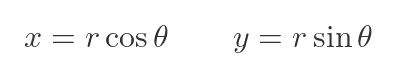
How do we find the derivative of x with respect to y, when all we know is ir r and θ? Well, we know how to convert from polar coordinates to Cartesian coordinates, using these well-known equations:

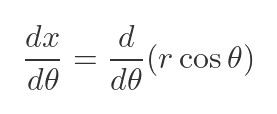
So we can differentiate x with respect to θ:

Remember that r is a function of θ. This means that our derivative is the product of two functions of θ, so we can use the product rule:

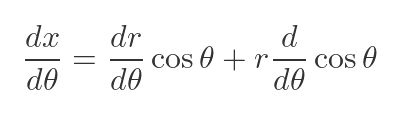
We can differentiate the cosine term:

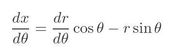
r is a function of θ, so assuming we can find its derivative (which will also be a function of θ), we now know the derivative of x in terms of θ.

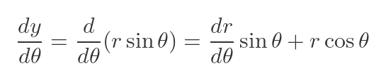
We can do the same thing to differentiate y wrt θ. We won't go through it in detail, it is very similar to the x case. Here is the result:

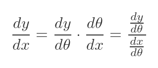
We can find the slope of the curve like this:

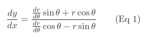
Substituting our previous values for the derivatives gives:

Finding the normal to a polar curve

The normal to a curve at any point is always perpendicular to the tangent. The normal is shown here in blue:

In general, the slope of the normal to a curve is the negative reciprocal of the slope of the tangent at the same point. In terms of the derivative, the normal has slope:

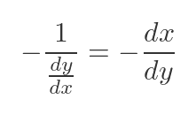
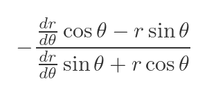
Based on the previous value for the derivative, this can be expressed as:

Polar curves often have vertical tangents, as in the example above. This happens when the denominator of the derivative goes to zero. In those cases, it can sometimes be useful to use the normal instead.

Example - tangent to a circle

Let's illustrate this with a very simple polar function:

With this function, r is always 1, for any value of θ. This, of course, creates a circle of radius 1:

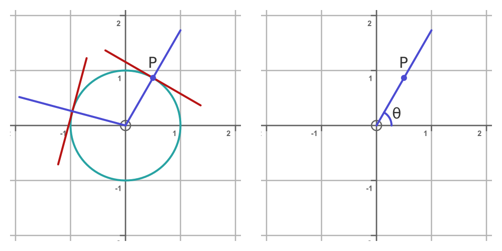
This LHS diagram also shows the tangent (red) and normal (blue) for two points on the circle.

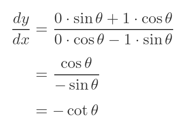
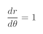
To find the tangent, we first note that, since r is constant, its derivative is zero:

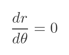
If we take our previous (Eq 1) for the slope, and substitute 1 for r and 0 for the derivative of r, we get a much simpler equation:

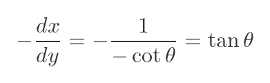
The normal is the negative reciprocal of the tangent:

We can check that this makes sense. We know from basic geometry that the normal to the circumference of a circle passes through its centre. The graph above also confirms that.

We also know that any point P can be expressed in polar coordinates as (r, θ), where θ is the angle that P makes at the origin. This is shown of teh RHS of teh graph above.

Based on these two facts, we can say that the normal to the curve at any point P has an angle θ, therefore it has a slope of tan θ. This is consistent with our expression for the normal to a circle in polar form.

Example tangent to a spiral

This polar function creates a spiral:

Since r is equal to θ, as θ increases, the curve gets further and further away from the origin. The LHS below shows this curve, with the tangent shown for θ of π/3. The tangent is at quite a steep angle, so for clarity, the black dashed line shows θ of π/3:

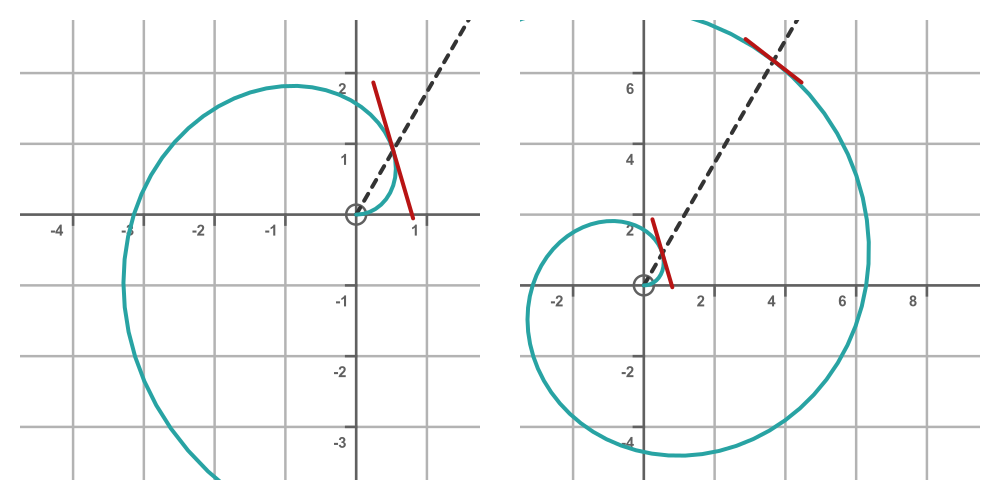
One thing to notice about the spiral function is that it is not cyclic. So, for example, θ values of π/3 and 7π/3 give different values of r, even though both angles look the same on the polar plot. This is shown on the RHS above. We can find infinitely many angles that are equivalent to π/3, simply by adding integer multiples of 2π. And as the diagram shows, they can have different tangents.

This time, since r = θ, the derivative of r is simply 1:

Again, we use our previous (Eq 1), substituting θ for r and 1 for the derivative of r. The tangent is:

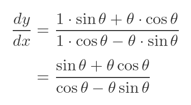
This equation includes terms that depend directly on θ (rather than the sine or cosine of θ), which is why it is not cyclic.

Example tangent to a cardioid

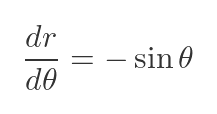
Now let's return to our cardioid curve:

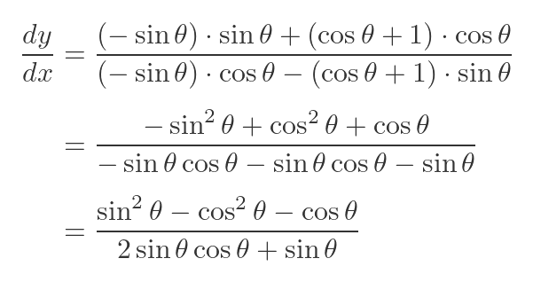
We saw the graph of this function earlier. We find the tangent using the same process as before. This time the derivative is:

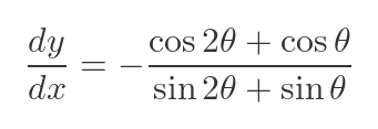
Substituting this into (Eq 1) gives:

We can simplify this formula using the following standard trig identities:

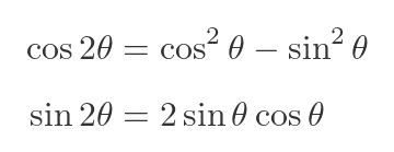
This gives a slightly nicer expression:

Related articles

• Standard curves in polar coordinates
• Polar curve constant r
• Polar curve constant theta
• Polar curve r proportional to theta
• Area under a polar function