Differentiation from first principles - x²

When we differentiate a function f(x) we obtain its derivative f'(x). The derivative is a function that tells us the slope of the curve for any value of x.

In this article we will see how to differentiate a function from first principles. This is a general technique that can be used to find the derivative of many different functions.

We will illustrate the technique for the specific case of x squared.

We will also derive the same result based on a geometric interpretation of the square function.

Differentiation from first principles

Here is a function f(x):

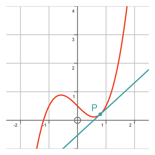
The slope of the curve at a particular P is given by the tangent to the curve at that point. The tangent is a line that just touches the curve without crossing it.

Finding the approximate tangent

We can find the approximate value of the tangent at point P by creating a second point Q, a small distance h further along the curve:

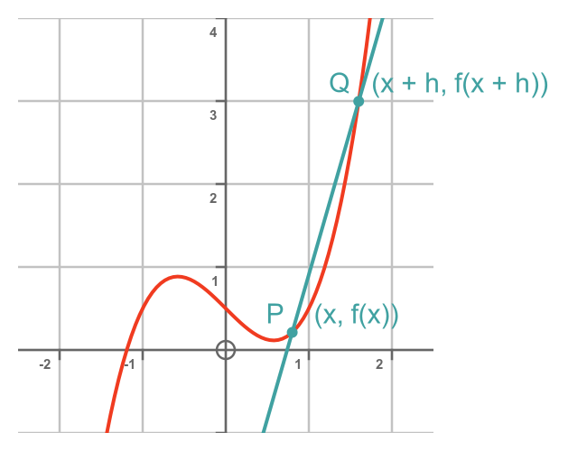
The line PQ has a slope that is approximately equal to the slope of the curve a P.

Point P has an x-value of x, so its y-value is f(x):

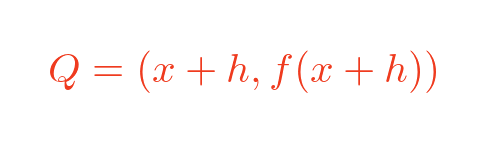
Point Q has an x-value of x + h, where h is some small value. Its y-value is f(x+h):

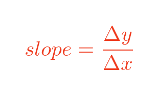
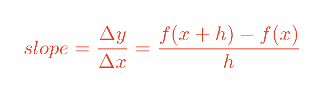
The slope of the line is given by:

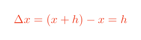
Where Δx, the change in x-values between P and Q, is:

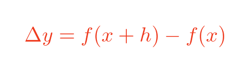
And Δy, the change in y-values between P and Q, is:

So the slope of PQ is:

Finding the exact tangent

The calculation above is only an approximation of the slope. The problem is that it measures the gradient of the line between P and Q. In fact, P and Q have been deliberately placed quite far apart to make it clear that the slope is not accurate.

But what we really want to know is the gradient of the tangent at the point P.

One thing we can do is move point Q closer to point P. This makes the slope PQ more similar to the slope at P:

The x-distance between P and Q is equal to h, so the smaller we make h, the closer the points become so the more accurate the slope.

But we can't simply set h equal to zero. If we did that, P and Q would be the same point. Δx and Δy would both be zero, so the slope would be zero divided by zero, which is undefined - it could be any value. So setting h to zero tells us nothing about the slope.

What we can do is evaluate the slope as h gets closer and close to zero. This is called a limit. As h gets closer to zero, the ratio of Δy and Δx often approaches a limiting value. We call this limit dy/dx (pronounced "dee y by dee x"):

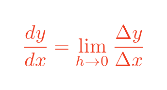
This notation tells us that dy/dx is equal to the limit of Δy over Δx as h tends to zero. This is equal to the slope of the tangent at x, so dy/dx is the derivative of f(x).

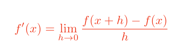
If we substitute the previous values for Δy and Δx we get:

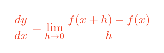
This is the derivative of f(x) from first principles.

We can also write this using prime notation, where we use f' to represent the derivative of f. So this equation means exactly the same thing as the previous one:

Now this formula doesn't tell us anything specific on its own, because we haven't yet specified what the function f(x) is. We will use the example of the x squared function, and use the formula to find the slope of that curve.

Differentiation x squared from first principles

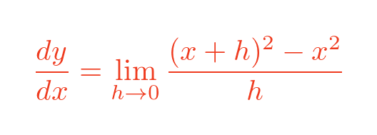
To differentiate x squared from first principles, we use the formula from before:

We then substitute x squared for f(x):

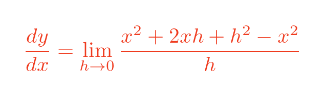
Multiplying out (x + h) squared gives:

The terms in x squared cancel out:

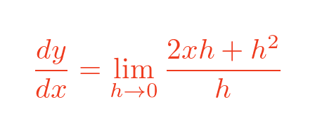
We can then cancel out a factor of h on the top and bottom:

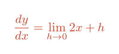
The limit is then quite simple. As h tends to zero, the h term just disappears, giving:

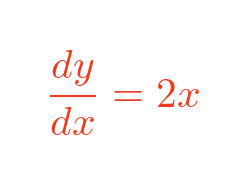
So at any point on the x squared curve, the slope is just 2 x.

Verifying the result graphically

Here is a table showing the slope of the curve for various values of x, using the formula 2x for the slope:

x	f'(x) = 2x
-2	-4
-1	-2
0	0
1	2
2	4

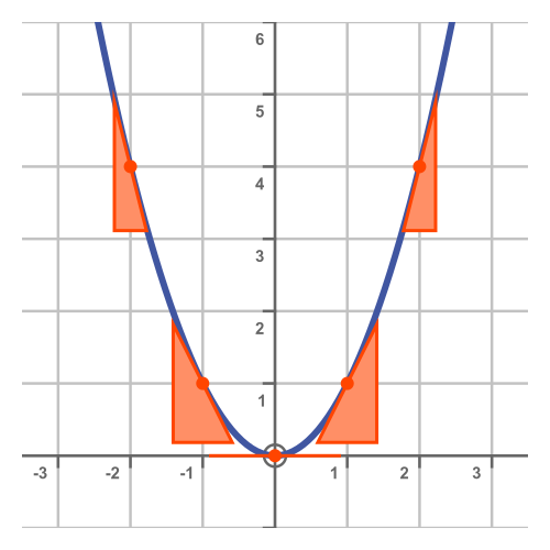
Here is a plot of x squared with tangent lines at x-positions -2 to +2, with the slopes calculated in the table. The slopes appear to match the slope of the curve:

Geometric interpretation

Finally, we will look at a simple geometric interpretation of differentiating x squared. The square on the left has sides of length x so its area, of course, is x squared:

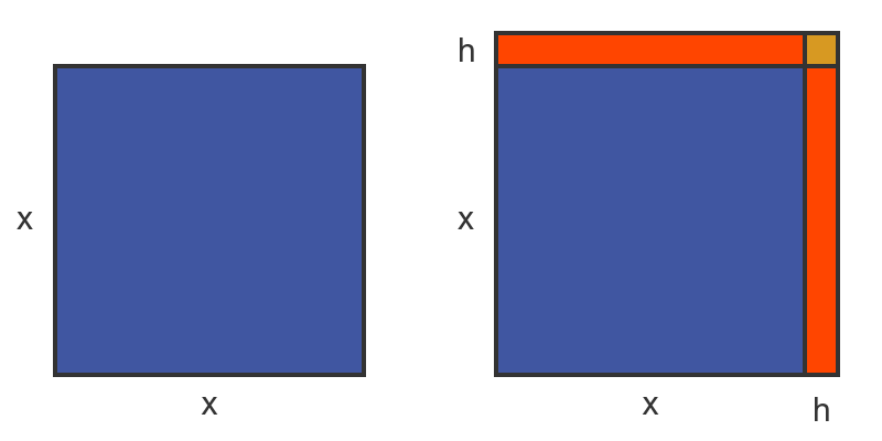
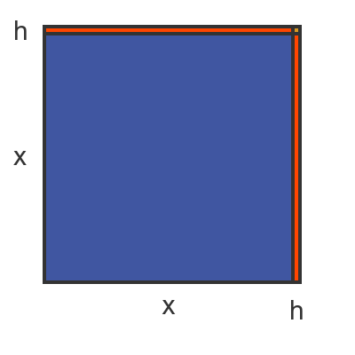
The square on the right shows what happens if we increase the side length of the square by a tiny amount h. This increases the total area of the square:

• It adds two rectangles to the square (shown in orange), each of size x by h. The total increase in area due to both of these rectangles is 2xh
• It also adds a small square (shown in yellow) of side h. This adds an extra area h squared.

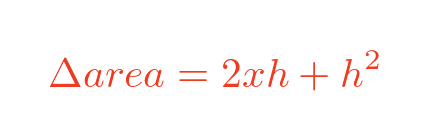
So the change in area, Δarea, of the square after increasing each side x by a small amount h is:

This looks quite similar to the earlier formula. Now let's see what happens as we make h smaller:

The two orange rectangles get smaller, but the tiny yellow square gets much smaller, much more quickly. As h gets extremely small, the yellow square becomes so small we can ignore it altogether. This removes the term in h squared:

So if we look at the rate of change of the area, which is Δarea divided by h, we get:

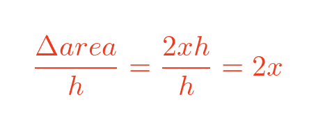
Which is the same result we found previously. This is a different way of looking at the same problem, which hopefully provides an intuitive explanation as to why we ignore the term in h squared.

See also

• Slope of a curve
• Differentiation from first principles - a to the power x
• Second derivative and sketching curves
• Differentiation - the product rule
• Differentiation - the quotient rule
• Differentiation - the chain rule
• Derivative of sine, geometric proof
• Differentiation - L'Hôpital's rule