Finding the normal to a curve

We know how to find the tangent to a curve using differentiation. How can we find the normal to a curve? In this article, we will see how to do this for a simple parabola x squared, and for an ellipse defined by a parametric equation.

What is the normal to a curve?

We can find the slope of a function at some point P by differentiating the function at that point. This gives us the instantaneous gradient of the curve at point P.

If we draw a straight line with that gradient that passes through P, it will form a tangent to the curve at P.

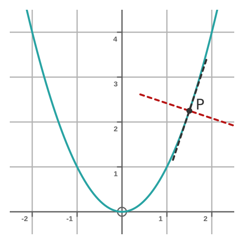
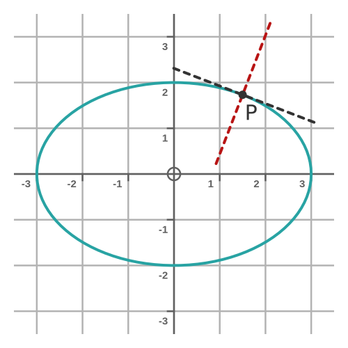
The normal to the curve is the line passing through P that makes a right angle with the tangent. This is shown here:

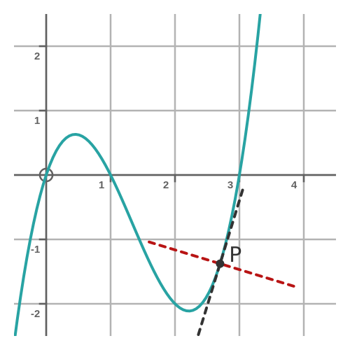
Here, the black dashed line is the tangent, and the red dashed line is the normal.

Finding the tangent to a parabola

We will start by looking at how we might find the tangent to the following simple parabola:

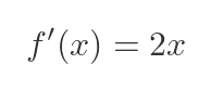
We can find the gradient of the parabola at any point by differentiating the function. This is a standard result for the x squared function:

We want to find the equation of the tangent at any point P. The tangent is shown as the black dashed line here:

The general equation for a straight line is:

Here, mp is the gradient of the line, and cp is the intercept (which we will need to calculate). The reason we are calling these quantities mp and cp (rather than m and c) is that every point P has a different tangent.

Since the line is a tangent, its slope must equal the gradient of the parabola at P:

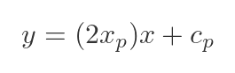
Putting this back into the straight line formula gives:

To find cp, we can use the fact that the curve passes though P, which has coordinates (xp, f(xp)). We can substitute these values for x and y:

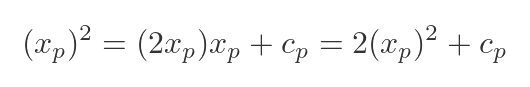
We can solve for cp:

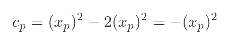
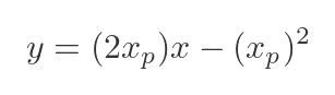
This gives us a formula for the tangent line, for any value xp

Finding the normal to a parabola

As we saw earlier, the normal to a curve at P is the line that passes through P at a right angle to the tangent. But we also know, from basic coordinate geometry, that the product of the gradients of any two perpendicular lines is -1. In other words, if a line has gradient m, the perpendicular line has gradient -1/m.

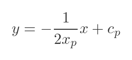
This means that the gradient of the normal will be -1/(2xp) rather than 2xp. The formula for the normal line is then:

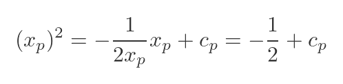
The normal passes through the same point P, so we can use the same technique to find cp:

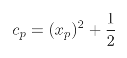
Solving for cp:

Which gives us this equation for the normal line at P:

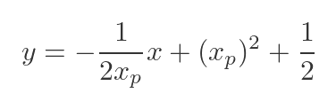
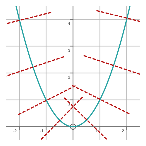
This is shown as the red dashed line on the previous graph. The graph below shows some more normals of the same function:

A parametric ellipse

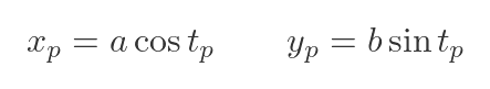
An ellipse is a slightly different situation. The ellipse curve is multivalued, so it is often expressed as a pair of parametric equations, like this:

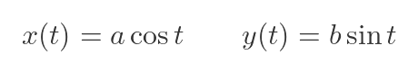
These formulas represent an ellipse that has its major and minor axes aligned with the x and y axes. It has a radius of a in the x-direction, and b in the y-direction. For illustration, we will use values 3 and 2 for a and b.

For any value t, the point (x(y), y(t)) will be on the circumference of the ellipse. If we take every value of t from 0 to 2π, it will trace out the entire ellipse. Here is the ellipse:

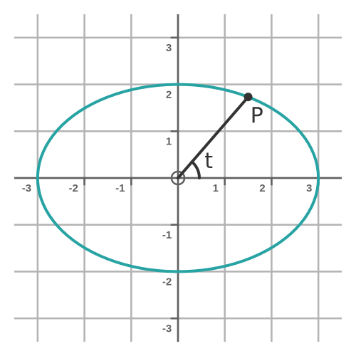
Notice that P makes an angle t with the x-axis.

Tangent to an ellipse

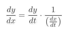
To find the tangent, we need to find the gradient of the ellipse function. In this case, we only know x and y in terms of t, but we can use the identity to find the gradient dy/dx:

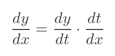
Essentially, we can manipulate derivatives in a similar way to ordinary fractions, because a derivative is just the limit of an ordinary fraction. This means we can also flip dt/dx:

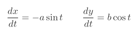
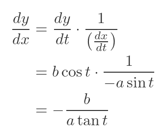
Now we have the gradient in terms of derivatives of x and y with respect to t. We can find these derivatives easily, because we already know x and y in terms of t. Differentiating the previous expressions gives:

Substituting these into the formula for the gradient gives:

This gives us the slope in terms of t. For example, at the point P in the diagram (when t is π/3) the slope is:

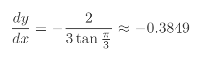
We won't calculate cp for the tangent here, because we only need the gradient to be able to find the normal.

The tangent (black) and the normal (red) are shown here:

Normal to an ellipse

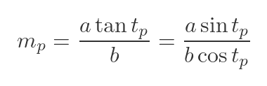
As before, if the slope of the normal is the negative reciprocal of the slope of the tangent. So the slope of the normal at P (where t = tp) is:

Again, since the normal passes through P. We can find cp in the same way as before:

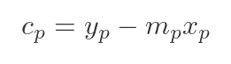
This time, of course, xp and yp are functions of tp:

Substituting the known values and simplifying gives:

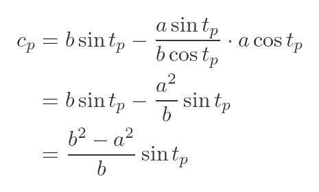
This gives a final formula for the normal to an ellipse at any point P:

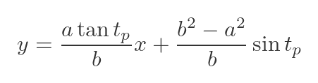
Those look quite complicated, but everything in the equation, apart from x and y, is a constant.

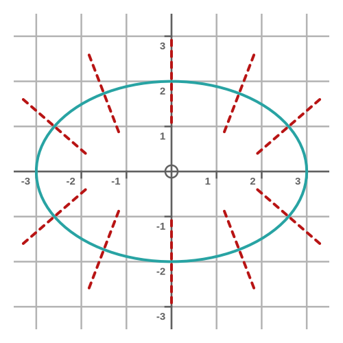
This graph shows various normals to the ellipse, calculated for different values of P:

A sanity check - normal to a circle

A circle, of course, is just a special type of ellipse. Specifically, it is an ellipse where the major and minor axes (a and b above) are equal.

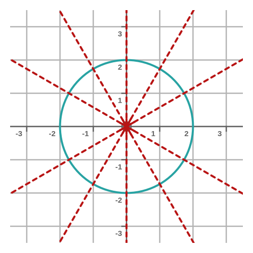
We also know, from basic geometry, that any radius of a circle is perpendicular to the tangent at the point where it crosses the circumference. This means that any normal to a circle must also be a radius, and therefore must pass through the centre of the circle. Here are some of the normals of a circle:

What does the ellipse formula tell us? We have just seen that the normals to an ellipse have the equation:

For a circle, a = b. Here is the equation when we replace set a and b equal (ie if we replace b with a everywhere in the equation):

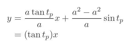
This shows that the normal lines have the form y = mx. When x is zero, y is also zero, so every normal to the circle passes through the centre of the circle (which is at the origin). This is consistent with our previous observation, that every normal to circle is collinear with a radius of the circle.

Related articles

• Slope of a curve
• Differentiation from first principles - x²
• Second derivative and sketching curves
• Differentiation - the product rule
• Differentiation - the quotient rule
• Differentiation - the chain rule
• Differentiation - the chain rule (proof)
• Differentiation - derivative of an inverse function
• Differentiation from first principles - a to the power x
• Derivative of ln x
• Derivative of sine, geometric proof
• Derivative of tangent
• Differentiation - L'Hôpital's rule
• Limits that fail L'Hôpital's rule