Fundamental theorem of calculus

The 2 main operations of calculus are differentiation (which finds the slope of a curve) and integration (which finds the area under a curve). The fundamental theorem of calculus relates these operations to each other. They are, essentially, inverses of each other (after taking account of the constant of integration).

There are 2 parts to the theorem. The first fundamental theorem of calculus shows that integration is essentially the inverse of differentiation, in other words, it is the antiderivative. The second fundamental theorem of calculus shows how to calculate definite integrals.

First fundamental theorem of calculus

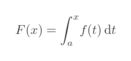
We write the definite integral of a function like this:

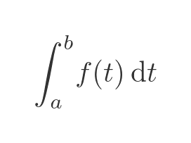
We have expressed this using the variable t rather than x, for reasons that will become clear in a moment. It doesn't matter what name we use for the variable, of course, the value of the definite integral remains the same.

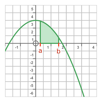
The definite integral represents the area under the curve between t = a and t = b, shown here:

Now suppose that rather than using a constant value b for the upper limit, we make the upper limit variable. We will call it x. Then the value of the definite integral becomes dependent on x. That is to say, as the value of x changes then the upper limit moves so the area under the curve changes.

So we can express the integral, ie the area under the curve, as a function of x:

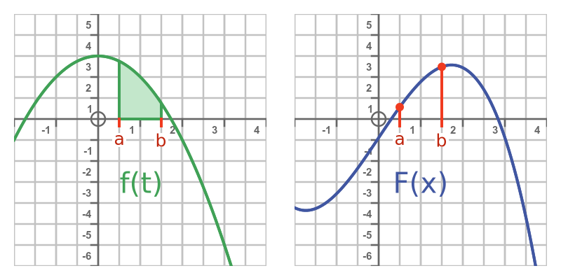
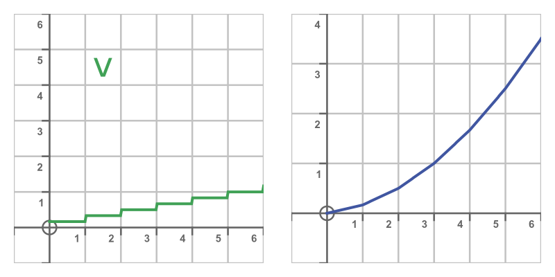
This idea is illustrated below. The left-hand curve shows the function f. The right-hand curve shows F. whose value is equal to the area under the curve on the graph of f:

Since F(x) represents the integral of f(t) from some arbitrary point a up to x, it means that F is, in effect, the indefinite integral of f.

Now we get to the important part, the theorem itself. This theorem doesn't automatically follow from what we have said so far, it needs to be proved (as we will do shortly) The theorem can be stated as:

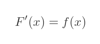
This tells us that, if F is the integral of f, then f is the derivative of F. This important theorem links differentiation and integration.

It tells us that the integral of f is equal to the antiderivative of f, where the antiderivative is the function you can differentiate to get f. This means that integration and differentiation are inverse processes.

This animation shows the slope of F compared to the area under f as x increases:

Notice that:

• Starting from x = a the slope of F is positive because f is positive.
• The slope decreases to zero as f approaches 0 (at approx 1.7).
• As x increases beyond that point, the slope of F becomes negative.

Second fundamental theorem of calculus

The second theorem relates to evaluating a definite integral. It tells us that:

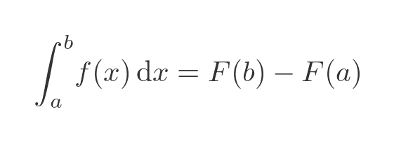
Here, again, F is the antiderivative of f. This is an important equation. It allows us to calculate the area under the curve f, between points a and b, simply be evaluating the antiderivative F for the two values a and b:

Finding antiderivatives

These theorems highlight a common feature of integration that we all learn fairly early when we start calculus.

It is often possible to find the derivative of a function from first principles, but that is rarely possible for integrals. Most of the known standard integrals have been discovered by reversing a known derivative.

For example, if we want to integrate an expression such as:

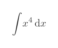
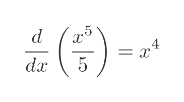
We need to already know an applicable antiderivative. In this case, we know that:

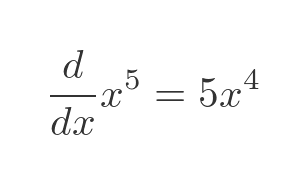
So we can find the thing that we need to differentiate to get x to the power 4:

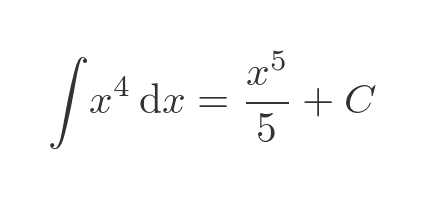
Which allows us to solve the integral:

Distance/velocity example

As an intuitive example, consider a trolley rolling along a flat surface, in a straight line, like this:

This trolley is travelling at a constant velocity, v, of 1 metre per second. So after 6 seconds, it will have travelled a distance, s, of 6 m:

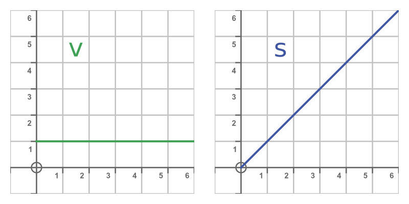
In this simple example, the slope of the distance graph is equal to the value of the velocity graph. We don't need calculus to work that out, it is the basic equation of motion for constant velocity.

Now let's consider the case of a trolley that changes its velocity over time. It starts with a low velocity, then after 2 seconds the velocity makes a step change to a higher value, and then after 2 more seconds it makes a step change to an even higher value:

The speed and distance graphs now look like this:

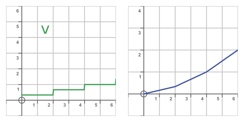
If you look closely you can see that the distance graph has 3 linear sections. In each section, the slope of the distance graph is equal to the magnitude of the velocity graph.

If we change the motion so that the velocity changes in 6 steps, the graph looks like this:

This time the distance graph has 6 linear sections, again with a slope that is equal to the value of the velocity at that time. But this time the linear sections are less pronounced.

It is easy to imagine that, if we continued to increase the number of steps until the velocity function was smooth, then the slope of the distance curve would still match the value of the velocity curve at every point in time.

Proof of the first theorem

We previously looked at quite a loose definition of the first theorem. We can state it more precisely here. If f(x) is a function that is continuous over the interval [a, b], we can define F(x) as:

The theorem states the for x in [a, b], the following is true:

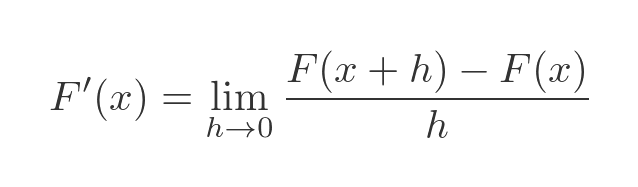
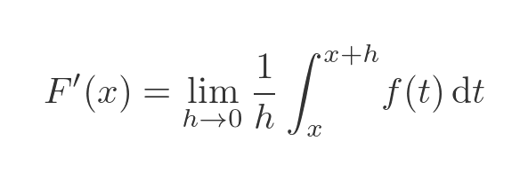
Let's start with the standard definition of the first derivative:

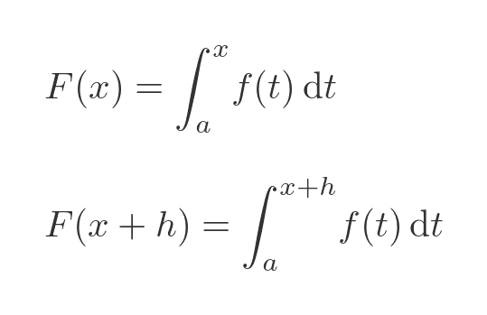
From the previous definition of F(x) we have:

We can substitute these terms into the derivative equation:

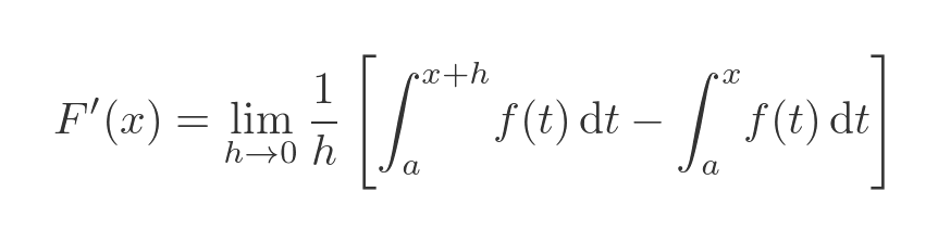
If we look at the two definite integrals, one has a range from a to (x + h), the other has a range from x to a. If we subtract one from the other we are left with the integral from x to (x + h):

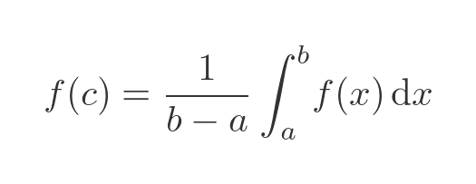
We can apply the mean value theorem for integrals to this formula. This theorem tells us that, if f(x) is continuous over the interval [a, b], then there will be a value c in [a, b] for which:

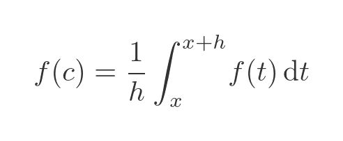
In our case, a is equal to x, and b is equal to (x + h), so of course (b - a) is just h. So we can apply the mean value theorem to give:

So we can write F'(x) like this:

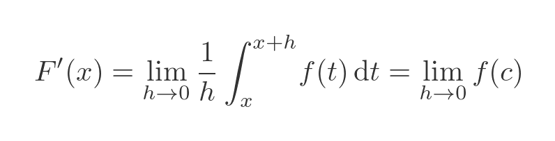
As we noted earlier, the mean value theorem says that c is in the interval [a, b], which in our case is the interval [x, x + h]. As h tends to 0. this interval tends towards [x, x], so in the limit, c tends to x. So we have:

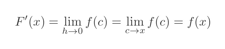
Which proves the theorem.

Proof of the second theorem

Again we will start by giving a more rigorous statement of the second theorem: if f(x) is a function that is continuous over the interval [a, b], and F(x) is any antiderivative of f(x) then the definite integral can be found from:

As an aside, notice that this applies to any antiderivative of f(x). This is because if F(x) is an antiderivative of f(x), then adding any constant of integration C to F(x) also yields an antiderivative of f(x). But because we are subtracting F(a) from F(b), any constant term will vanish.

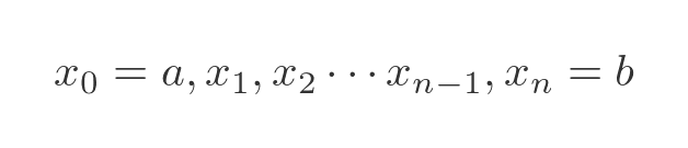
To prove this theorem, we will start by dividing the interval [a, b] into n equal sub-intervals, like this:

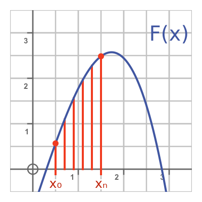
Boundary 0 is at a, boundary n is at b, and boundaries 1 to (n - 1) are equally spaced between them:

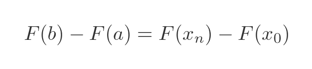
Using this scheme, we can express the RHS of the original equation as:

Now we will do a little trick:

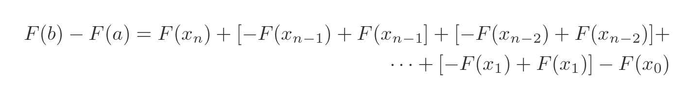
Notice what we have done here. We have added two terms in (n - 1), one negative and one positive, so they cancel out to 0. We have also added two terms in (n - 2), one negative and one positive, which also cancel out to 0. And so on. Since all the extra terms cancel out, this equation is identical to the previous one.

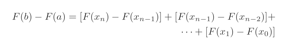
So now we can group these terms differently (this is the same expression as before, we have just shifted the brackets around):

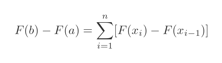
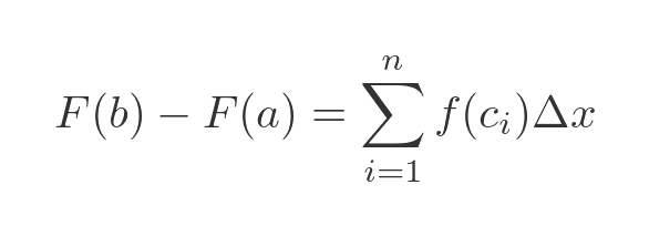
The reason for doing all this is to allow us to write it as a sum:

Next, we are going to use the mean value theorem. This is closely related to the mean value theorem for integrals we used earlier, and it states that there exists some value c in the interval [u, v] for which the following is true:

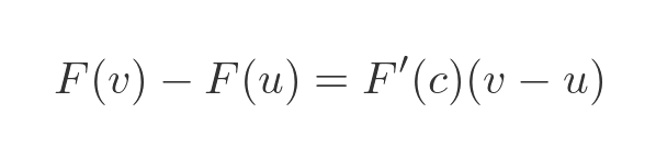
We can apply this to each one of the terms under the sigma above:

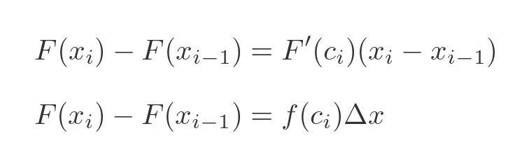
We have simplified this in the second line, by substituting f(x) for F'(x) (we know they are equivalent from earlier). And also since all the x values are equally spaced we can just use Δx for the difference (it doesn't depend on i). So the sum of all these terms is:

This sum is equal to the sum of the areas of these rectangles:

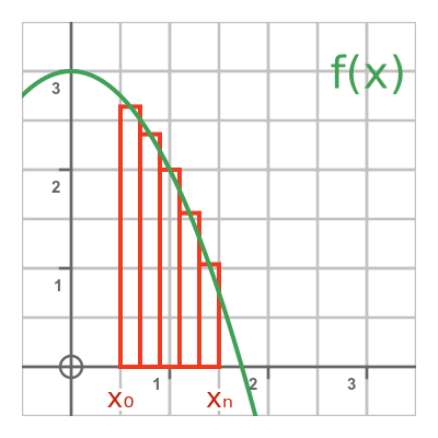
As n increases towards infinity, Δx goes to 0, and the area will tend towards the definite integral of f(x). This proves that:

See also

• What is integration
• Integration by substitution
• Mean value theorem for integrals
• Integration by parts
• Finding arc length by integration
• Gabriel's horn