Normal distribution

The normal distribution is a standard probability density function (PDF) that is often used to model random distributions. It is also known as the Gaussian distribution.

In this article, we will recap what a PDF is, and why it is useful to model distributions with a standard distribution. We will then look at the characteristics of normal distribution and investigate some ways we can use it in real life, including the use of the central limit theorem.

Probability density functions

The normal distribution is usually used to represent continuous, real-valued random variables. For example:

• If we measured the heights of individual people in a population, we could represent these as a PDF. If we then selected an individual at random, the density would tell us the probability that the height of the random individual was within a certain range.
• If we recorded the times of a particular athlete throughout many 100m races, they could also be represented as a PDF. This could be used to estimate the probability that the time of their next race would be between, say, 10.2 and 10.5 seconds.

Taking the second example, here is what the probability density might look like for an athlete running 100m:

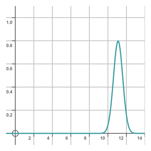
We can think of this, loosely, as representing how likely the athlete is to achieve a particular time in any given race. This shows they are most likely to achieve a time close to about 11 seconds, with some chance of doing 10.5s on a good day or 11.5s on a bad day, and a much smaller chance of doing 10s or 12s on a really good or bad day. This range is a little unrealistic, we are only using it for the purposes of illustration. Someone who normally takes 11s is unlikely to achieve 9.5s no matter how good a day they are having!

A more accurate interpretation is to say that the probability of the time being between a and b is equal to the area under the curve between a and b:

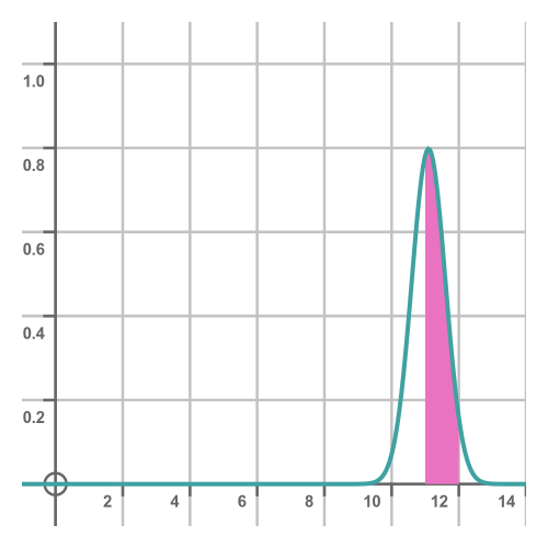
In this case, the shaded area gives the probability that the time will be between 11s and 12s. A probability density function is always calculated so that the total area under the curve is exactly 1, because the total area under the curve represents the probability of any possible outcome. Since there always had to be exactly one outcome, the area under the curve must be 1.

A consequence of this definition is that the probability of the outcome being exactly equal to some value v is zero. The area representing a range of exactly v would have zero width, therefore zero area, therefore zero probability.

This makes sense if you think about it. The probability of the time being in the range of 11 to 12 is quite high. The probability of it being in the range of 11 to 11.1 is obviously quite a bit lower. The probability of it being in the range of 11 to 11.01 is even lower. And so on. If we keep on making the range smaller, the probability of the time being within that range gets smaller. If the range is zero, the probability will go to zero.

Modelling a distribution

We can find the actual distribution of real data by sampling it and generating a histogram. However, that can also be advantages to modeling a real distribution using an idealised mathematical function.

While the model function might not be an exact fit for the real data, it might well be close enough for all practical purposes. The model function has the advantage that it will usually have nice mathematical properties because the function will have been chosen with that in mind. There will also be well-known, standard results that you can apply to your data because many other people have used the same model in the past. It might also make it easier to compare your data with other data sets that have also been modelled with the same standard distribution.

The normal distribution

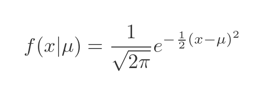
The normal distribution is probably the most well-known and widely used PDFs. The standard function is:

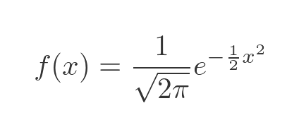
This function is based on the exponential function of x squared, so it is symmetrical about the y-axis. It looks like this:

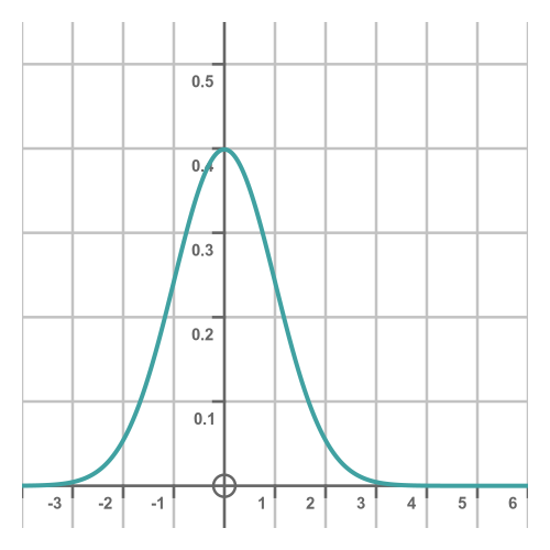
If you are wondering about the constants:

• The divisor of root 2π is there to ensure that the total area under the curve is equal to 1. This is a requirement for any PDF as mentioned earlier.
• The factor of one-half in the exponent ensures that the standard deviation of the PDF is 1.

So the basic normal distribution has a mean of 0 and a standard deviation of 1. The standard deviation is a measure of how spread out the data is. If the standard deviation is small, most of the values will be close to the mean. If it is larger, the values will be spread out more. This is illustrated later.

Fitting the normal distribution to real data

Suppose we had some real-life data that appeared to be a bell shape, but its mean value isn't 0, instead it was some value we will call μ (the Greek letter mu). We can adapt the normal distribution like this:

The notation here is to add μ as a parameter, separated by a bar. This means that f is a function of x that we are defining assuming a certain value of μ.

All we have done here is to replace x with x - μ, which of course shifts the whole curve by μ in the x direction. For example, here we are using a value of 2 for μ:

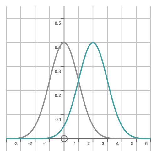
Since we have only shifted the curve along by μ without changing its shape, the standard deviation will be the same.

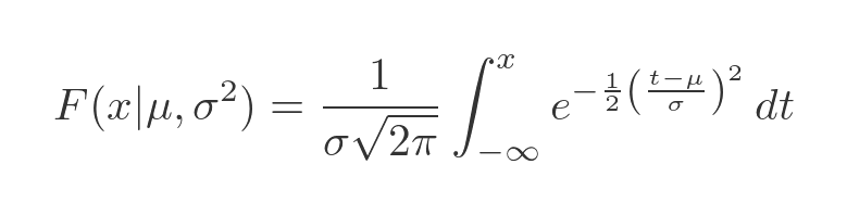
What if our data had a different standard deviation? If it was more or less spread out than the default standard deviation? Let's call the new standard deviation σ (the Greek letter sigma). We won't prove it here, but we can adjust the distribution function like this:

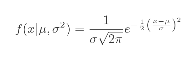
This time we have added the parameter σ squared to the function definition. If you are wondering why the term is squared, it is because the square of the standard deviation is called the variance, which is an alternative measure of spread. Traditionally the normal distribution is defined based on its mean and variance, so we use sigma squared as the second parameter of the distribution.

Here are the normal curves with standard deviations of 0.8 (the blue curve) and 1.4 (the orange curve):

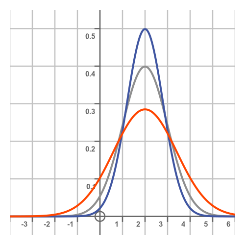
Notice that a larger standard deviation makes the spread of the distribution wider, but it also makes the central peak smaller. This follows from the fact that the area under each curve is the same, exactly 1, so if the curve is wider it can't be as tall. Another way to view this is that a larger standard deviation means that samples are more likely to be found further from the centre, which means they are less likely to be found close to the centre.

Advantages of the normal distribution

The normal distribution has a symmetrical bell shape, that is often seen in real-life distributions. It is a continuous function with some well-known properties:

• The mean, median and mode of the distribution are all the same, all occurring at the central peak of the curve.
• The shape of the curve is entirely controlled by the two values μ and σ. The curve can be fitted to any data that has a similar bell-shaped curve with a known μ and σ.
• The distribution has a known cumulative distribution function (CDF) which is an important function that allows us to calculate the probability of a sample being within a certain range.
• Regardless of μ and σ the distribution follows the 68–95–99.7 rule, that approximately 68% of samples will be within +/-σ of the mean μ, 95% will be within +/-2σ, and 99.7% will be within +/-3σ.

Finally, the central limit theorem allows us to combine two independent normal distributions to obtain a single distribution that is also a normal distribution.

Probability of sample being within a certain range

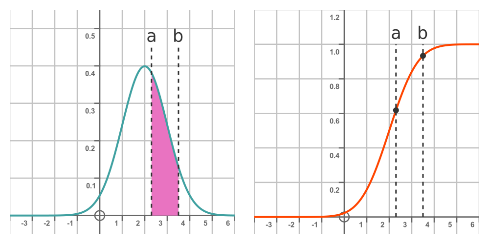
Given a normal distribution, we know that the probability of a random sample being less than some value b is given by the area under the PDF from minus infinity up to b. This is shown by the graph on the left:

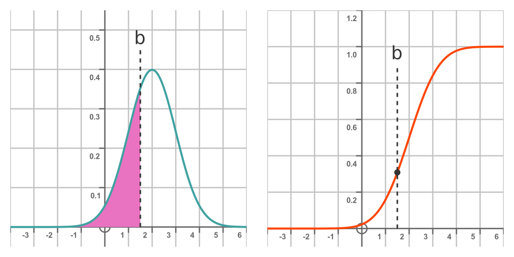
The graph on the right shows the CDF mentioned earlier. We will call this function F(x). It is the integral of the PDF from minus infinity to the point of interest, b. So the value of the CDF at b is the probability that a random sample with be less than b. In other words:

There is no closed solution to this integral, but there are various ways to evaluate it numerically to any required accuracy. We won't go into details here. Many calculators can calculate this as normalcdf or similar, and the functionality is available in most programming languages.

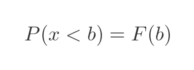
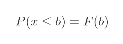
So we can now say that the probability of x being less than b is F(b):

And since the probability that x is exactly b is zero, the probability of x being less than or equal to b is the also F(b):

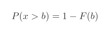
The probability that x is greater than b is one minus the probability that x is less than b, since x must either be less than or greater than b (again since the probability of them being equal is zero):

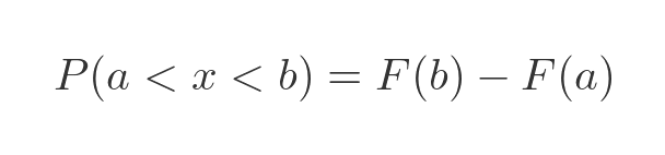
Finally, what is the probability that x is between two values a and b? Well, assuming a < b, it will be the difference in areas between the curve to b and the curve to a:

In terms of the CDF, this is:

Combining normal distributions

If we have two independent random variables that both have normal distributions, the sum or difference of those variables will also have a normal distribution. And we can calculate the mean and standard deviation of the sum or difference.

As an example, suppose a small business makes an average income of £5000 a week, with a standard deviation of £500. The business outgoings (rent, stock, utilities etc) are £4000 a week with a standard deviation of £600. We will assume sales and outgoings are independent of each other.

If the profit of the business is equal to income minus outgoings, what would the distribution of the weekly profits be?

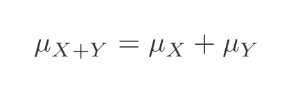
Well, as noted earlier, it would be a normal distribution, so we can apply some standard rules. If we have two independent random variables X and Y, then the mean of the sum of those variables will be the sum of the means:

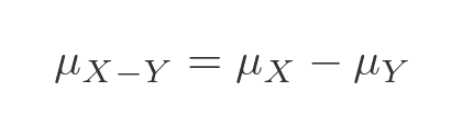
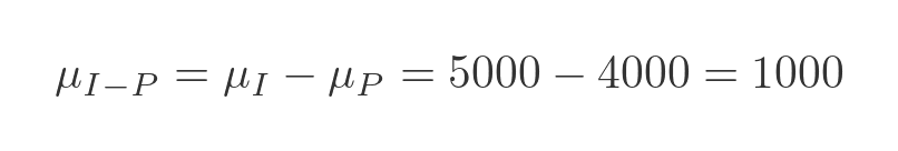
The mean of the difference of those variables will be the difference of the means:

To calculate the combined standard deviation, we need to use the variance, which is equal to the square of the standard deviation. The variance of the sum of those variables will be the sum of the variances of each variable.

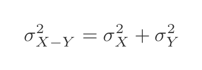
What about the variance of the difference of the two variables? Well, this might seem a little counter-intuitive, but the variance of the difference of those variables will also be the sum of the variances of each variable. When we combine two variables the variance always goes up, whether we add or subtract them. Having two random variables at play makes things more random! So we have this formula:

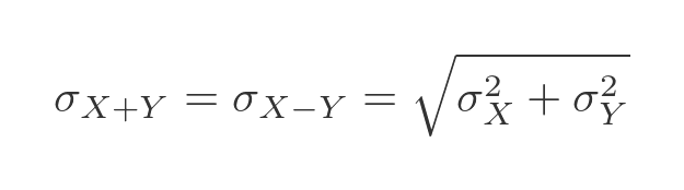
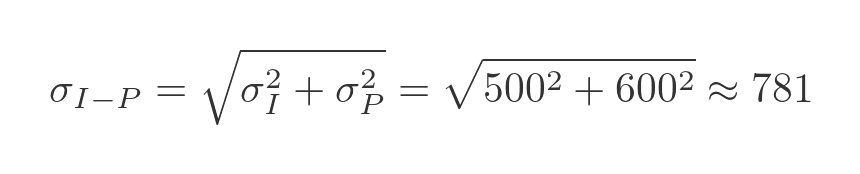
We can find the standard deviation by taking the square root:

Using the figures above, the mean weekly profit of the business will be the mean income minus the mean outgoings:

The standard deviation of the weekly profit is:

See also

• Binomial distribution