Binomial distribution

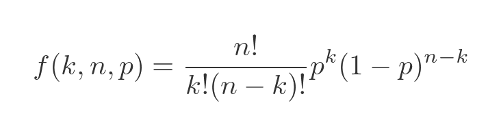
Suppose you rolled a fair dice, ten times. What is the probability that you would throw a six exactly three times?

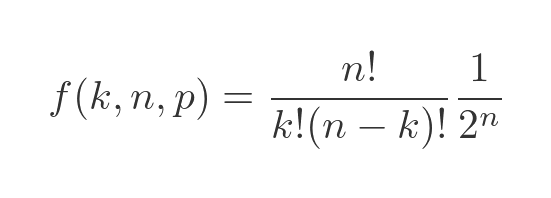
This situation can be modelled by a binomial distribution so the result can be found using the probability mass function of the binomial distribution. The formula is stated here, but we will look at this in more depth in a little while:

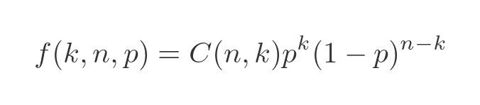
In this article, we will find out what a binomial distribution is, and how to use the formula to solve problems like the one above. We will see where the formula comes from, and see some of the properties of the distribution.

Binomial distribution

The binomial distribution is a discrete probability distribution, which means it applies to a series of separate trials. In our example above, each roll of the dice counts as a trial. A trial is some kind of process that has two possible outcomes, succeed or fail. In our case, we say the trial succeeds if the dice comes up six, and fails if it is any other number.

In the formula above:

• n is the total number of trials we will perform. In our case, we intend to roll the dice ten times.
• k is the number of passes we are expecting. In our case, we are calculating the probability of exactly three passes (ie rolling a six on three occasions out of the ten attempts).
• p is the probability of the success of each trial. In our case, success means rolling a six, so p is 1/6 with a fair dice.

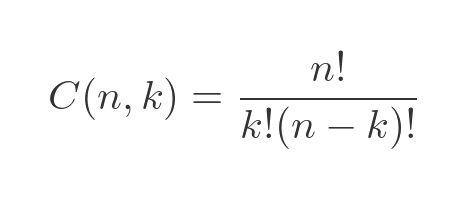
What about C(n, k)? That is the binomial coefficient, given by:

This gives a final formula for the probability of:

This might seem like quite a complex formula for what is a fairly simple concept, but we will break it down shortly.

But first, how does it apply to our original problem? Remember n is 10, k is 3, and p is 1/6. Substituting these values into the equation gives:

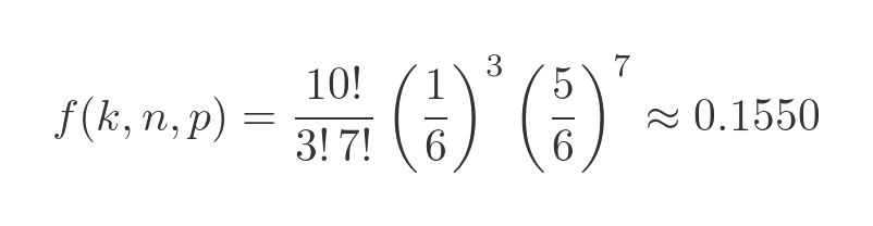
So the probability of getting exactly three sixes in ten throws of the dice is about 15%. Intuitively, that seems reasonable. You expect to get a six every six throws, on average, so getting three of them in ten throws is a little unlikely but certainly not impossible.

Conditions for applying the Binomial distribution

As we saw earlier, the Binomial distribution function f(k, n, p) tells us the probability that, if we conduct n trials, where the probability of success is p, exactly k of those trials will succeed.

But there are a few other conditions that must be satisfied.

• The number of trials must be fixed. In our case, we have already decided to throw the dice ten times, so that condition is met.
• Each trial must be independent. In our case, we throw a fair dice each time, so the previous results can't affect the next result, so that is fine.
• The probability of success must be the same for every trial. Since it is a fair dice, the probability of throwing a six is always the same, so again that is fine.

To give some examples of how these conditions might be broken, consider these situations:

• We might decide that, rather than throwing the dice ten times, we will keep throwing the dice until we throw a two. Now we no longer have a fixed number of trials. We can't use the Binomial distribution directly to find the probability of throwing three sixes before we throw a two, because we don't know how many throws that will be.
• We might deviate from simply throwing the dice each time. For example, we might decide that if the dice comes up with the same number as the previous throw, we will ignore that throw and try again. This means that the trials are no longer independent because the result of one trial can affect the next trial.
• Instead of using a dice, we might use a bag full of counters, each with a number between one and six. Instead of throwing the dice each time, we take a random counter out of the bag and we don't put it back in the bag afterwards. In each trial, one of the counters is removed from the bag, so in the next trial the probabilities of drawing each different number will change. If we take out a three, for example, then on the next trial there is less chance of drawing a three and therefore more chance of drawing something else.

This isn't to say that it would be impossible to work out the probabilities in the cases above, but we can't use the Binomial distribution to do it.

Plotting the binomial distribution

In our example, we used a fair dice, and rolled it ten times. We calculated the probability of getting three sixes. But what about other results? The probability of getting two sixes, no sixes, or maybe even ten sixes? We can calculate these values using the previous formula:

We use the same values of 10 for n, and 1/6 for p, but we vary k. This tells us the probability of rolling k sixes if we throw ten fair dice. Of course, we can only calculate this for certain values of k. For one thing, k must be an integer, because we can't roll a six 0.5 times. And of course, k must be between 0 and 10 inclusive because we can't get -1 sixes (that makes no sense), or 11 sixes (because we are only throwing the dice ten times).

If we calculate the value of the formula for all the possible k values, we get a graph like this:

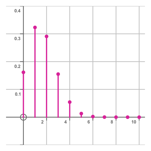
This tells us that the most likely number of sixes is one, closely followed by two. That makes sense because we would expect to get a six, on average, every six throws. So after ten throws, we would most likely get one or two sixes. zero and three are also reasonably likely. Higher numbers are less likely, and the probability of throwing ten sixes is very small indeed.

This is called the probability mass function. Why is that? Well, many other probability distributions are continuous (for example, the normal distribution). In a continuous distribution, we calculate the probability of the random value being in a certain range using the area under the curve. For example, for the following normal distribution, the probability of the value being between 11 and 12 is given by the shaded area:

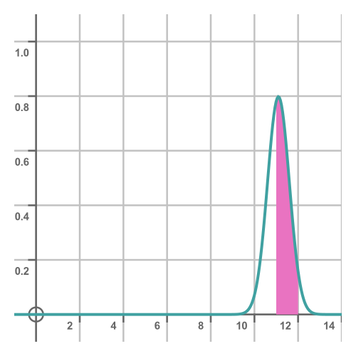
For a discrete distribution, there is no area to calculate. The probability is only defined for certain values. Rather than having the probability distributed over an area, it is all concentrated into specific places, as if those were point masses.

The cumulative distribution function

The mass function tells us the probability of getting a particular number of sixes. But we might also want to know the probability of getting, for example, three or fewer sixes. The cumulative distribution function (CDF) tells us that. Here is the CDF for ten throws of a dice:

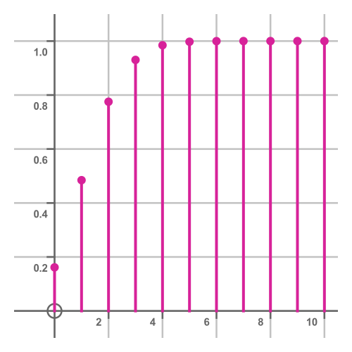
Notice that the CDF approaches 1 as k increases. When k is 10, the CDF is exactly 1 because this represents the probability that the number of sixes will be less than or equal to ten. Since the number of sixes can't be greater than ten, the probability that it is less than or equal to ten must be exactly 1.

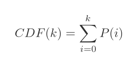
The CDF is quite easy to calculate. If P(k) is the probability of the result being exactly k, then CDF(k) is found by adding all probabilities from P(0) to P(k):

Another example - flipping coins

Now let's quickly look at another example. What is the expected outcome if we toss a fair coin, twenty times?

We will arbitrarily decide that a coin coming up heads counts as a success, and tails is a fail. It doesn't make too much difference because, of course, the probability of heads is 0.5, and the probability of tails is 0.5. So we have n as 20 and p as 0.5.

Here is what the probability mass function looks like. We simply plot the previous function with the new parameters, noting that the possible number of heads is any integer in the range 0 to 20:

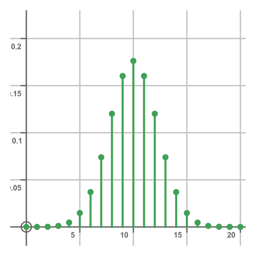
This main difference compared to the previous plot is that the probabilities of success and failure are equal, whereas, in the case of the dice, success was less likely. This means that the average value of the plot is in the centre and the curve is symmetrical rather than being skewed as in the dice case.

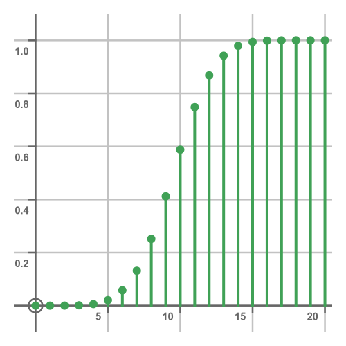
Here is the equivalent CDF, again calculated as the running sum of the probability masses:

Properties of binomial distributions

Let's look at some properties of binomial distributions, starting with the mean. The first thing we should do is clarify what we mean by the mean, so to speak.

In our example, a trial is one roll of the dice. The binomial distribution describes ten trials. We will call this an experiment - an experiment means performing ten trials, and the result of that experiment is the number of sixes that were thrown in those ten trials.

To find the mean of the distribution, we might perform lots of experiments, record the result of each experiment, and then find the mean average of all those experiments. After many experiments, we would discover the mean. The mean is the average number of successes per experiment, averaged over many experiments. But there is an easier way - we can calculate the mean. In general, the mean of any discrete distribution will be:

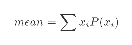
Here xi represents all the possible outcomes, so it has values 0 to 10. P(xi) represents the probability of each outcome. In other words, we take the value of every possible outcome and multiply it by the probability of that outcome occurring. If we add all those products together, it gives us the mean value of the distribution. This can be simplified for binomial distribution with parameters n and p. We won't prove it here (it will be the subject of a later article), but it simplifies to:

This equation makes sense intuitively. Each time we roll the dice, there is a probability of p that it will land on six, and that probability is 1/6. So, after the ten trials that make up an experiment, on average we would expect six to appear 10/6 times, or approximately 1.6667.

The mode is the value with the highest probability. This can be found from the probability mass function:

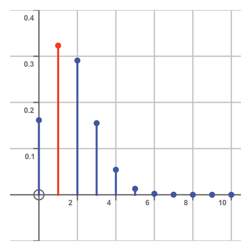
The mode in this case is one. The outcome of an experiment is more likely to be one than any other value.

For a discrete distribution, the median is the smallest value, m, which satisfies:

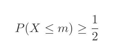
In other words, if we pick a random value x from the distribution, there is a 50% or greater chance that x is less than or equal to m. The CDF represents the probability of x being greater than or equal to a particular value. So we can find the median by drawing a line on the CDF graph at 0.5:

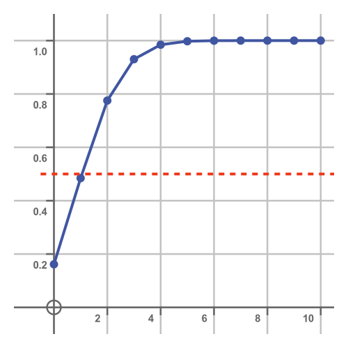
The smallest x value where the CDF goes above this line is 2, so that is the median. We have ignored the pathological case where there are several x values with a CDF of exactly 0.5, which is unlikely to occur with a binomial distribution.

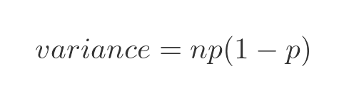
The variance of a binomial distribution can be found using the usual formula - the mean of the squares minus the square of the mean. Again we will not prove it here, but for a binomial distribution this reduces to:

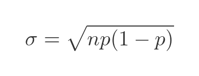
The standard deviation is defined as the square root of the variance:

Where does the binomial distribution formula come from?

We have been using this formula for the probability mass function:

But where does this come from? It is best to think of the formula as being in two parts. Remember that, for any particular distribution, n and k are fixed so the only variable is k. For each value of k:

• The first part of the formula (the bit with the factorials) gives the total number of possible results that have exactly k successes.
• The second part (the two probabilities) gives the probability that any one of those possible results occurs.

Multiplying these two terms together will give us the overall probability of an experiment producing k successes (remember that an experiment involves performing n individual trials).

We will use two examples to justify this equation. First, a simplified coin example, where n is reduced to 3. Then the full dice scenario from earlier.

Coin justification

If we toss a fair coin three times, there are eight possible outcomes. Each of the three coins can be either a head or a tail. Two (the number of options) raised to the power three (the number of coins) is eight. Since there aren't that many possibilities, we can list them all:

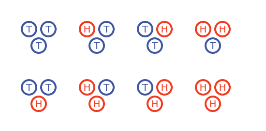
What is the probability of getting exactly two heads (k equals 2)? Well, we can see that three possible results have exactly two heads. These are HHT (throwing two heads followed by a tail), HTH, and THH. And we also know that any of the eight possible combinations is equally likely. So the probability of throwing two heads is the number of possible results that have two heads (which is three) divided by the total number of possible results (which is eight). So it is 3/8.

That is all fine if we have a small number of coin tosses. But if we wanted to do the calculation based on twenty throws, there are over a million different combinations. Drawing them all out and counting them would be quite tedious.

Coin toss probabilities using C(n, r)

If we look at the three cases where there are two heads, they are HHT, HTH, and THH. Why are there three cases? Well, of course, that is because there are three different ways of ordering two heads and one tail.

What if we had four coins, two of which are heads? Then there would be six possibilities - HHTT, HTHT, HTTH, THHT, THTH, TTHH. These are the six different ways of ordering two heads and two tails.

We can generalise this. The total number of ways of ordering n coins where k are heads, and the rest are tails is given by C(n, k). That is the total number of combinations of k items picked from n, and is sometimes described as choose k from n. We previously saw this was:

We then divide by 2 to the power n because that is the number of possible orderings of n coins, and each ordering is equally likely:

But this only works when p is 1/2, as we will see next.

Dice justification

Returning to our example of throwing a dice ten times, how many combinations of three items are there? If we use "6" to indicate a six was thrown, and "X" to indicate a non-six, we have combinations such as XXXXXXX666, XXXXXX666X, XXXXXX66X6, and so on. The total number of such combinations is C(10, 3) which evaluates to 120.

What is the probability of getting one of those combinations? Well, in the case of the coins, we simply divided the number of combinations by the total number of possible outcomes.

But we can't do that here! That calculation was based on the assumption that all possible outcomes are equally likely, That is true for tossing a coin, but not for rolling a six on a dice. The combination XXXXXXXXXX (ie ten non-sixes) is reasonably likely (from the graph of the dice probability function, the probability of rolling no sixes is about 0.16). But the combination 6666666666 is almost impossible (the odds are about one in ten million).

To resolve this, we need to take another look at the coin calculation. We previously took the C(n k) value and divided it by 8 because that is the number of equally likely possible outcomes.

But we could look at it slightly differently. We could take the C(n k) value and multiply it by the probability of that particular outcome occurring. What is the probability of getting HHT in three flips of the coin? We can break it down like this:

• The probability of getting a head in the first flip is 1/2.
• The probability of getting a head in the second flip is 1/2.
• The probability of getting a tail in the final flip is also 1/2.

We multiply these probabilities together to get the probability of all three happening, which gives us 1/8. And the probability of getting HTH or THH is also 1/8, by the same logic. This is the same result as before - we divide C(n, k) by 8 - but derived in a different way.

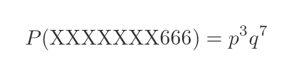
Now let's apply this to the dice problem. We will use p to indicate the probability of getting a 6, which of course is 1/6. We will use q to indicate the probability of getting anything other than 6. This is (1 - p), or 5/6.

What is the probability of throwing XXXXXXX666 in ten throws? Well each 6 had a probability of p, and each X has a probability of q, so our final probability is formed from the product of three p terms and seven q terms:

The probability of getting XXXXXX666X is the same because again it is formed from the product of three p terms and seven q terms, just in a different order. This applies to every combination of three sixes. Since there are C(10, 3) possible ways of throwing three sixes, the probability of getting this result is:

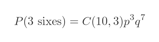
The reason there are three p terms is that k is 3, and the reason there are seven q terms is that n - k is 7, so we can rewrite this in terms of n, p and k:

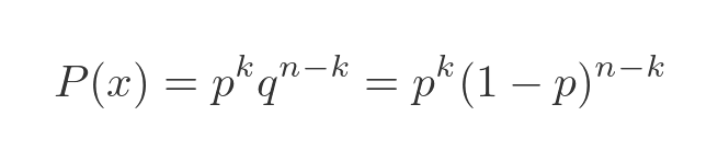
Generalising to any n and k gives us the probability mass function from earlier:

See also

• Normal distribution