Solving equations numerically
Categories: numerical methods pure mathematics
In this section we will look at exactly what we mean by solving an equation, why we might need to use numerical methods to solve an equation.
We will only consider functions of one variable, denoted by $f(x)$.
Solving an equation f(x) = 0
When we solve an equation, we are finding the values of $x$ for which $f(x)$ meets a particular condition. A common type of equation is:
$$ f(x)=0 $$
In this case we want to find the values of $x$ for which $f(x)$ is zero. For example:
$$ x^3 - 2x^2 -x + 2 = 0 $$
Here is a graph of this function:

In this case the polynomial can be factorised quite easily as:
$$ (x + 1)(x - 1)(x - 2) = 0 $$
Solutions to this equation are -1, 1, and 2.
Solving an equation f(x) = c
A second type of equation has the form:
$$ f(x)=c $$
Where $c$ is some constant value. This can be rewritten in the form:
$$ g(x)=0 $$
Where:
$$ g(x) = f(x) - c $$
For example the equation:
$$ x^2 + 2x - 2 = 1 $$
Can be rewritten as
$$ x^2 + 2x - 3 = 0 $$
As shown in this graph:
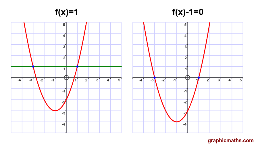
The left had graph shows the solutions to $f(x)=c$, the right hand graph shows the solutions to $g(x)=0$. In both cases the solutions are -3 and 1.
Solving an equation f1(x) = f2(x)
A third type of equation has the form:
$$ f1(x)=f2(x) $$
In this case we need to find the values of $x$ for which the two formulas have equal values. This can be rewritten in the form:
$$ h(x)=0 $$
Where:
$$ h(x) = f1(x) - f2(x) $$
For example the equation:
$$ x^2 + 2x - 2 = 2 - x^2 $$
Can be rewritten as
$$ 2 x^2 + 2x - 4 = 0 $$
As shown in this graph:
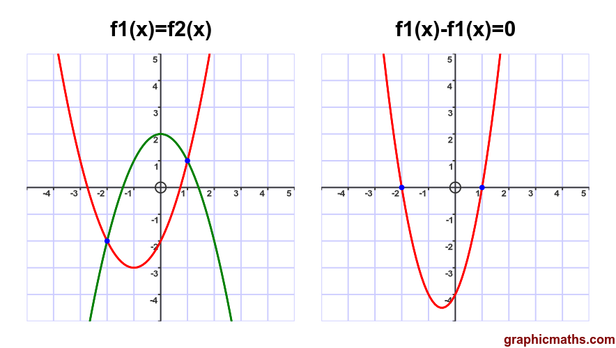
The left had graph shows the solutions to $f1(x)=f2(x)$, the right hand graph shows the solutions to $h(x)=0$. In both cases the solutions are -2 and 1.
Solving an equation algebraically
In some cases it is possible to find an exact solution for an equation algebraically, for example by rearranging the formula to solve for x:
$$ \begin{align} x^2 = 2\newline x = \sqrt 2 \end{align} $$
Or factorising:
$$ \begin{align} x^2 + 2x - 3 = 0\newline (x + 3)(x - 1) = 0\newline x = -3, 1 \end{align} $$
Or using inverse functions
$$ \begin{align} e^x = 3\newline x = \ln 3 \end{align} $$
Not all equations can be solved in this way. For example, polynomials of degree 5 or higher cannot generally be solved exactly using algebra. In those cases we can use numerical methods.
Numerical methods
A numerical method is an algorithm that can be used to find an approximate solution to an equation. Most methods use a form of trial and error:
- Starting with an initial trial value for the solution.
- Calculate how inaccurate the trial value is (the error).
- Use a defined method to finding a new trial value that is better than the previous value.
- Check accuracy of the result and repeat from step 2 if necessary.
Since this method gives a numerical answer, it is often only an approximation. However, in most cases it is possible to achieve any required degree of precision by repeating the procedure a sufficiently large number of times. This will normally be done by computer, of course, and for many problems an ordinary PC will be able to calculate an answer to 16 significant figures in a fraction of a second.
For simplicity, most numerical methods work with equations of the form $f(x)=0$. As we have seen, it is easy to convert other types of formula to this form.
It is always useful to have a reasonable idea of how many solutions the equation has, and roughly where the solutions are. If possible it is best to sketch the graph before you start.
Accuracy of result
In most cases, we will need to check the accuracy of the result to decide if the current result is accurate enough, or if we need to continue looping to gain more accuracy. There are several ways to check the accuracy of the current solution $x$:
- We can check the value of $f(x)$. Usually, the closer the this value is to zero, the closer $x$ is to the solution.
- We can check previous estimates of $x$. If current value and previous value differ by less then 0.1, the value is likely to be accurate to about 1 decimal place. If they differ by less than 0.01, the result is likely to be accurate to about 2 decimal places, and so on.
These techniques assume that the function behaves approximately like a straight line when we get close to the solution. This is the case with a lot of mathematical functions - the more we zoom in on a particular part of the function, the more it looks like a straight line. However, if you are dealing with a function that doesn't behave like that, extra care is needed to ensure that the solution is accurate.
Related articles
Join the GraphicMaths Newsletter
Sign up using this form to receive an email when new content is added to the graphpicmaths or pythoninformer websites:
Popular tags
adder adjacency matrix alu and gate angle answers area argand diagram binary maths cardioid cartesian equation chain rule chord circle cofactor combinations complex modulus complex numbers complex polygon complex power complex root cosh cosine cosine rule countable cpu cube decagon demorgans law derivative determinant diagonal differential equation directrix dodecagon e eigenvalue eigenvector einstein ellipse equilateral triangle erf function euclid euler eulers formula eulers identity exercises exponent exponential exterior angle first principles flip-flop focus gabriels horn galileo gamma function gaussian distribution gradient graph hendecagon heptagon heron hexagon hilbert horizontal hyperbola hyperbolic function hyperbolic functions infinity integration integration by parts integration by substitution interior angle inverse function inverse hyperbolic function inverse matrix irrational irrational number irregular polygon isomorphic graph isosceles trapezium isosceles triangle kite koch curve l system lhopitals rule limit line integral locus logarithm maclaurin series major axis matrix matrix algebra mean minor axis n choose r nand gate net newton raphson method nonagon nor gate normal normal distribution not gate octagon or gate parabola parallelogram parametric equation pentagon perimeter permutation matrix permutations pi pi function polar coordinates polynomial power probability probability distribution product rule proof pythagoras proof pythagorean triple quadrilateral questions quotient rule radians radius rectangle regular polygon rhombus root sech segment set set-reset flip-flop simpsons rule sine sine rule sinh slope sloping lines solving equations solving triangles special relativity speed of light square square root squeeze theorem standard curves standard deviation star polygon statistics straight line graphs surface of revolution symmetry tangent tanh transformation transformations translation trapezium triangle turtle graphics uncountable variance vertical volume volume of revolution xnor gate xor gate