Solving equations using interval bisection
Categories: numerical methods pure mathematics

The previous article discussed using numerical methods to solve equations of the form $f(x) = 0$.
In this article we will look at one of the simplest methods, interval bisection.
Example problem
As a simple example, we will solve the equation:
$$x^2 - 2 = 0$$
This equation has a solution $x = \sqrt 2$ (and an second solution $x = -\sqrt 2$). We will only look for the first solution. Although we already know the answer to the problem, it is still useful to work through the numerical solution to see how it works (and to gain an approximate value for the square root of 2).
To use the technique we need to have a rough idea of where the solution is. It is useful to sketch a graph of the function:
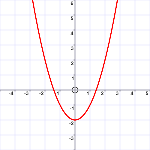
We need to specify interval (ie a range of $x$ values) that contains exactly one solution. It doesn't have to be extremely accurate. For example, it is obvious from the graph that a solution exists between values $x=1$ and $x=2$. We write an interval as $[1, 2]$, meaning every number between 1 and 2.
The process of interval bisection proceeds as follows:
- Start with an initial interval (1 to 2 in this case).
- Divide the interval into two equal halves.
- Determine whether the solution is in the lower half or the upper half.
- Repeat step two with the selected half.
Steps 2 to 4 are repeated until a sufficiently accurate result is obtained, as described in the solving equations article. On each pass, the interval width is halved, so the approximation becomes more accurate. When the result is accurate enough, the process ends.
A graphical explanation of interval bisection
To gain an intuitive understanding of the process, we will go through a couple of iterations and show the results on a graph. This is for illustration only, you don't need to draw an accurate graph to use this method.
First iteration
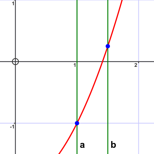
The first iteration starts with an interval $[1, 2]$. Here is the graph where we have zoomed in to the region of interest. a shows the line $x = 1$ and b shows the line $x = 2$:
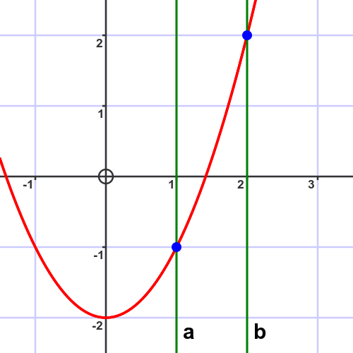
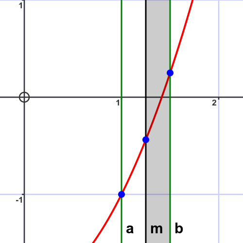
We now find the midpoint of the interval:
$$ m = (a + b) /2 = 1.5 $$
We use this to divide the original interval in half to create 2 intervals $[a, m]$ and $[m, b]$:
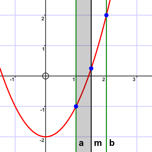
The solution of the equation is the point where the curve crosses the x-axis. In this case, the solution is in the lower interval $[1, 1.5]$.
Second iteration
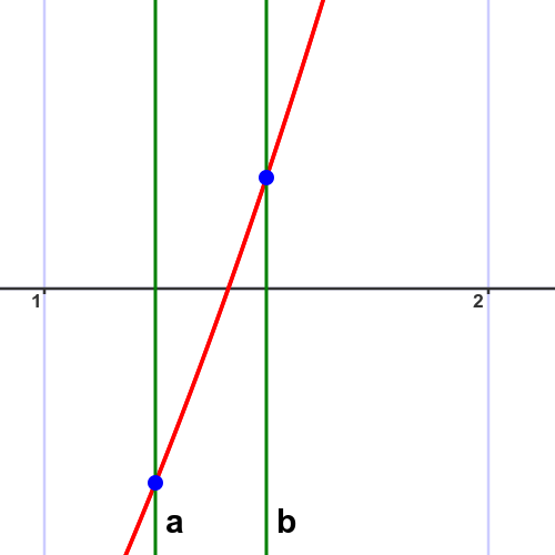
The second iteration starts with the new interval $[1, 1.5]$. Again, we have zoomed in further:
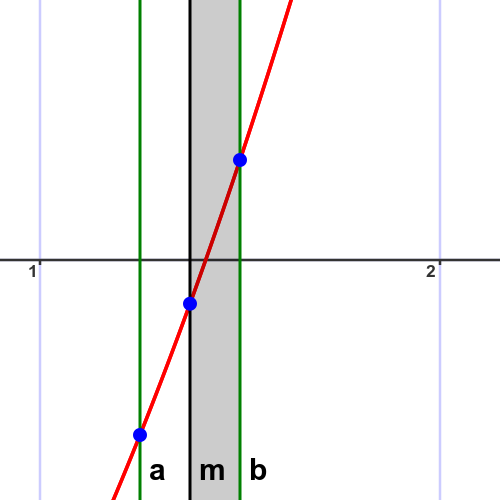
The new midpoint is 1.25:
This time the solution is in the upper interval $[1.25, 1.5]$.
Third iteration
The third iteration starts with the new interval $[1.25, 1.5]$:
The new midpoint is 1.375:
The solution is in the upper interval $[1.375, 1.5]$.
On each iteration, the width of the interval is halved, starting at 1, then 0.5, then 0.25. After 10 iterations the interval width will be about 0.00097, so we will have calculated the square root of 2 to about 3 decimal places. After 20 iterations we will know the answer to around 6 decimal places, and after 30 we will be accurate to around 9 decimal places. Although this would be tedious (but not impossible) to do manually, for a computer it would take almost no time at all.
Interval bisection by calculation
In the example above, we have relied on the fact that we have a very accurate graph of the function to determine whether the solution is in the first or second half of the interval. But is it possible to determine this by calculation alone. Of course, it is still useful to have an initial sketch graph to find a suitable starting interval.
For each iteration:
- Start with the current values of $a$ and $b$.
- Calculate $m$ as $(a + b)/2$
- Calculate the values of $f(a)$, $f(b)$, and $f(m)$.
- Based on the signs of $f(a)$, $f(b)$, and $f(m)$, determine if the solution is in $[a, m]$ or $[m, b]$.
- Repeat with the new range.
In this case, $f(x)$ is our function:
$$f(x) = x^2 - 2$$
Here is the calculation based on $a = 1$, $b = 2$
| a | b | m | f(a) | f(b) | f(m) |
|---|---|---|---|---|---|
| 1 | 2 | 1.5 | -1 | 2 | 0.25 |
Notice that $f(a)$ and $f(m)$ have opposite signs. This means that the root must be somewhere between $a$ and $m$.
For the second iteration, we therefore start with $a = 1$, $b = 1.5$ and calculate again:
| a | b | m | f(a) | f(b) | f(m) |
|---|---|---|---|---|---|
| 1 | 1.5 | 1.25 | -1 | 0.25 | -0.4375 |
This time, $f(b)$ and $f(m)$ have opposite signs. This means that the root must be somewhere between $m$ and $b$.
For the third iteration, we therefore start with $a = 1.25$, $b = 1.5$, and so on.
Related articles
Join the GraphicMaths Newsletter
Sign up using this form to receive an email when new content is added to the graphpicmaths or pythoninformer websites:
Popular tags
adder adjacency matrix alu and gate angle answers area argand diagram binary maths cardioid cartesian equation chain rule chord circle cofactor combinations complex modulus complex numbers complex polygon complex power complex root cosh cosine cosine rule countable cpu cube decagon demorgans law derivative determinant diagonal differential equation directrix dodecagon e eigenvalue eigenvector einstein ellipse equilateral triangle erf function euclid euler eulers formula eulers identity exercises exponent exponential exterior angle first principles flip-flop focus gabriels horn galileo gamma function gaussian distribution gradient graph hendecagon heptagon heron hexagon hilbert horizontal hyperbola hyperbolic function hyperbolic functions infinity integration integration by parts integration by substitution interior angle inverse function inverse hyperbolic function inverse matrix irrational irrational number irregular polygon isomorphic graph isosceles trapezium isosceles triangle kite koch curve l system lhopitals rule limit line integral locus logarithm maclaurin series major axis matrix matrix algebra mean minor axis n choose r nand gate net newton raphson method nonagon nor gate normal normal distribution not gate octagon or gate parabola parallelogram parametric equation pentagon perimeter permutation matrix permutations pi pi function polar coordinates polynomial power probability probability distribution product rule proof pythagoras proof pythagorean triple quadrilateral questions quotient rule radians radius rectangle regular polygon rhombus root sech segment set set-reset flip-flop simpsons rule sine sine rule sinh slope sloping lines solving equations solving triangles special relativity speed of light square square root squeeze theorem standard curves standard deviation star polygon statistics straight line graphs surface of revolution symmetry tangent tanh transformation transformations translation trapezium triangle turtle graphics uncountable variance vertical volume volume of revolution xnor gate xor gate