Vector drawing with generativepy

generativepy is an open-source Python drawing library that can create computer images, diagrams, and animations. It can be found on github. This article covers generativepy V50.00, although much of it will also apply to older or newer versions.

This chapter covers the basics of creating vector images with generativepy. It provides a simple template for drawing vector images using the drawing module. It also shows how to use the geometry module to draw various shapes and style them.

generativepy can also create bitmap images, NumPy-based images, 3D images, and videos. We cover these in later tutorials, but the basic process is similar in all cases.

Vector images

A computer image is often stored as a 2-dimensional array of pixels, where each pixel can be any colour. This is called a bitmap image.

However, with vector graphics, we don't usually specify the colours of individual pixels. Instead, we work at a higher level, defining shapes in the image. These can be simple shapes, such as rectangles, or more complex shapes, such as text characters.

When we use generativepy in vector mode, our program specifies a shape and how to fill and outline it. The generativepy library decides the colour of each pixel.

The result is still a bitmap image file, in PNG format. However, your code describes the image in terms of shapes rather than pixels, which is more useful for mathematical images.

In this article, we will look at:

• The generativepy coordinate system
• Drawing basic shapes (such as lines, polygons, circles, and more).
• Fill and outline styles.

Vector graphics also include more advanced features, such as compound shapes (e.g., shapes with holes), complex curves, and clipping. We will look at these in a later chapter. There are also specialised techniques for mathematical diagrams, such as creating geometric diagrams and graphs, which we will cover in a later chapter.

Creating our first image

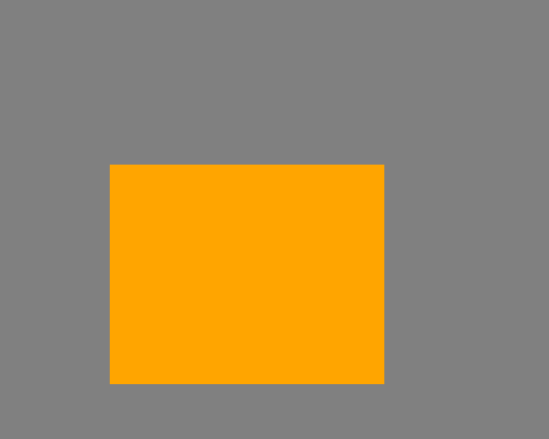
To start, we will create the following simple image, as a 500 by 400 pixel PNG file, consisting of an orange rectangle on a grey background:

Before you try this code, you will need to install generativepy and its dependencies, see the introduction

The code

Here is the code to draw the image above:

from generativepy.color import Color
from generativepy.drawing import setup, make_image
from generativepy.geometry import Rectangle

def draw(ctx, width, height, frame_no, frame_count):
    setup(ctx, width, height, background=Color("grey"))
    Rectangle(ctx).of_corner_size((100, 150), 250, 200).fill(Color("orange"))

make_image("rectangle.png", draw, 500, 400)

We will now look at this code in more detail.

Basic structure

The basic structure of the code is:

• A user-defined function draw that does the drawing.
• A call to make_image. This function creates an image and saves it to a file. We pass in the draw function to control the image content.

This basic structure is used throughout generativepy. We use a draw function to create the drawing, and a make_XXX function to create the image. We use the same pattern for bitmap images, NumPy-based images, and 3D images. We use the same pattern whether we are creating still images, animated GIFs, image sequences, or videos.

In all cases, images are stored in memory as "frames". A frame is a NumPy array containing the pixel data. This makes the library flexible, as you can combine images from different sources using simple Python and NumPy functions.

For vector images, like this one, generativepy uses the Pycairo library behind the scenes. In fact, ctx is a Pycairo drawing context.

make_image

The make_image function in the drawing module is the main function for creating vector images.

The parameters are:

• outfile, the filename of the output PNG file.
• A draw function that does the actual drawing.
• The width and height of the image in pixels.
• An optional channels parameter that is mainly used for creating images with transparency.

The draw function is one we define ourselves to draw the image. It doesn't have to be called draw, of course - you can call it whatever you like, provided you pass its name into make_image. The draw function must have the correct signature (in other words, it must accept the parameters described below).

draw function

The draw function draws the image content. We never call draw ourselves. We always pass draw into make_image, and make_image calls draw. The draw function accepts 5 parameters:

• ctx is a Pycairo context. This is like a virtual drawing surface that you can draw on in code. Whatever you draw will appear on the final image.
• width and height are the width and height of the image in pixels. These are the values that we passed into make_image.
• frame_no and frame_count are only used when you want to create image sequences (for animations), so we can ignore them here.

generativepy uses Pycairo as its drawing library. generativepy provides a rich set of high-level drawing functions for creating shapes, text, markers, graphs, and formulas that can be added to the image within the draw function

The generativepy drawing functions are built on top of the normal Pycairo functions. If you are familiar with Pycairo, it is also possible to use the Pycairo functions directly, or even to use a mixture of generativepy and Pycairo calls. Usually, though, it is better to stick with the generativepy functions as they operate at a higher level and are designed specifically for maths and diagrams.

Our draw function calls the setup function to set up the drawing area, then draws a rectangle.

setup function

The setup function isn't mandatory, but it does some useful things, so you will often want to call it.

setup has 3 required parameters: ctx, width and height. We use the values that were passed into the draw function. It has some optional parameters that do various things, described below.

In this case, we are setting the background parameter to Color("grey"), which sets the background colour to a mid-grey. We define the colour using the color module of generativepy. In this example, we are using colour names to select colours. These names are based on the CSS named colours. The color module has much more functionality, described in a later chapter.

Drawing a rectangle

We use a Rectangle object to draw a rectangle, like this:

Rectangle(ctx).of_corner_size((100, 150), 250, 200).fill(Color("orange"))

All shapes are drawn using the same pattern:

• Declare a shape object, for example Rectangle(ctx), passing in the context, ctx.
• An of_xxx method is used to define the shape. In this case, of_corner_size defines a rectangle from the position of its top, left-hand corner, and its width and height. The corner is specified using an (x, y) tuple.
• A drawing method is then used to draw the shape. In this case, we use fill, which fills the shape with orange.

Coordinate system

All coordinates and sizes are specified in user space coordinates.

By default, user space is measured in pixels, based on the size of the image we are creating.

• The origin of the user space coordinate system (0, 0) is at the top left of the image.
• x values increase from left to right.
• y values increase as you move down the image.

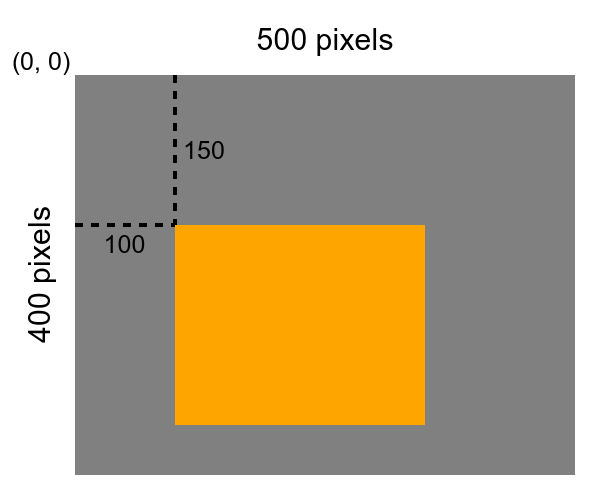
In our case:

• Our image is 500 by 400 pixels.
• The orange rectangle is 250 by 200 pixels.
• The position of the rectangle (that is, the position of its top-left corner) is at pixel position (100, 150).

This diagram illustrates the coordinates of the rectangle:

User space can be transformed, so that shapes drawn in user space can be scaled, rotated, etc when they are drawn, as we will see in a later tutorial.

Styling shapes

Now that we have seen how to draw a simple shape, we'll look at how to style shapes by filling and outlining them. This can add clarity to diagrams by using colour to link related items. Colour can also make your images more interesting and appealing.

Of course, when designing graphics we should always be aware that some of our intended audience might not be able to see colour differences clearly due to colour vision deficiency (so-called colour blindness) or other visual impairments. It is always a good idea to use light and dark colours, different shapes, dashed vs solid lines, and text labelling, in addition to pure colour, to make your diagrams accessible.

Filling shapes

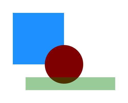
We have already seen how to fill a shape, but here is another example with 3 shapes:

Here is the code:

from generativepy.color import Color
from generativepy.drawing import make_image, setup
from generativepy.geometry import Rectangle, Circle, Square

def draw(ctx, width, height, frame_no, frame_count):
    setup(ctx, width, height, background=Color(1))

    Square(ctx).of_corner_size((50, 50), 200).fill(Color("dodgerblue"))
    Circle(ctx).of_center_radius((250, 250), 75).fill(Color("maroon"))
    Rectangle(ctx).of_corner_size((100, 300), 350, 50).fill(Color("green", 0.4))

make_image("fill.png", draw, 500, 400)

The Square object draws the large blue square. A square is created in a similar way to a rectangle, but it only has a width (unlike a rectangle that has a width and height).

The Circle object draws the purple circle. A circle is specified similarly to a square, except that the of_center_radius method takes a centre point and a radius value to define the circle.

The other thing to notice is that the circle overlaps the previous square. Because the square was drawn before the circle, the circle is painted over the square. Part of the square is hidden behind the circle. To draw the square in front of the circle, we would reverse the drawing order by swapping the two lines of code.

The green Rectangle object, lower down the image, overlaps the circle. This time the rectangle is painted over the circle. However, the rectangle colour is partly transparent, so we can still see part of the circle behind the rectangle. The rectangle colour is set to green, but the extra parameter 0.4 is the transparency value. Because the rectangle is partly transparent, we can see the red circle behind it.

You might also notice that the background colour in the setup function is Color(1). Using 1 rather than a colour name creates a grey value of 1, which is white (described in detail in a later chapter).

Shape outlines

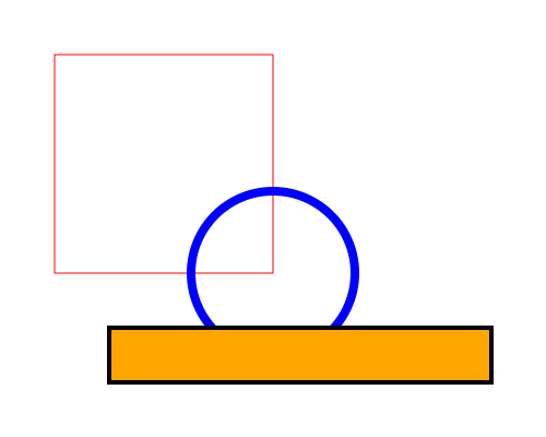
In addition to filling shapes, we can also outline them. We do this using the stroke method rather than the fill method. Here are the same shapes as before, outlined in different colours:

Here is the code:

from generativepy.color import Color
from generativepy.drawing import make_image, setup
from generativepy.geometry import Rectangle, Circle, Square

def draw(ctx, width, height, frame_no, frame_count):
    setup(ctx, width, height, background=Color(1))

    Square(ctx).of_corner_size((50, 50), 200).stroke(Color("red"), 1)
    Circle(ctx).of_center_radius((250, 250), 75).stroke(Color("blue"), 8)
    (Rectangle(ctx).of_corner_size((100, 300), 350, 50)
                .fill(Color("orange")).stroke(Color("black"), 4))

make_image("stroke.png", draw, 500, 400)

To draw a shape outline, we use the stroke method instead of the fill method. stroke requires two parameters: the colour and the stroke width. Width is measured in user space, so by default, the stroke width is specified in pixels.

The square has a red stroke colour and a width of 1 unit (i.e., 1 pixel). This draws a thin line around the square. The middle of the square is left unfilled.

The circle has a blue stroke colour and a width of 8. This makes a much thicker line. Again, the circle is not filled so we can see the outline of the red square behind it.

The final shape, the rectangle, is filled and stroked. We call fill with the colour orange, and stroke with the colour black and a width of 4.

We call fill before stroke, so that the rectangle is filled first, then outlined.

Fill and stroke position

The stroke follows the shape's outline, with half the stroked area inside and half outside. Here is an example of a filled and stroked rectangle:

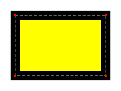
The dotted white line shows the outline of the rectangle, ie the exact size and position we requested. The 4 small red dots show the rectangle's corners. This indicates that the stroke is half outside the boundary and half inside.

This means that a stroked rectangle is always slightly bigger than its requested size because the stroke is centred on the exact boundary. And the filled area inside the rectangle is always slightly smaller than the requested size because the stroke covers part of the inner area. This is typical behaviour in most computer graphics systems and is intended. It looks best when, for example, the edges of two outlined shapes touch.

You can stroke the shape first and then fill it. In that case, the fill colour will occupy the whole area of the rectangle, and the stroke will appear to be half of its defined width. This method isn't used often, but it could be useful if you wanted to paint a shape at its exact size while still having an outline.

Join styles

There are some more options for styling line strokes. It is possible to style the way the lines join, using the join parameter of the stroke method:

from generativepy.color import Color
from generativepy.drawing import make_image, setup
from generativepy.geometry import Square, MITER, ROUND, BEVEL

def draw(ctx, width, height, frame_no, frame_count):
    setup(ctx, width, height, background=Color(1))

    (Square(ctx).of_corner_size((50, 50), 100)
                .stroke(Color("black"), 30, join=MITER))
    (Square(ctx).of_corner_size((200, 50), 100)
                .stroke(Color("black"), 30, join=ROUND))
    (Square(ctx).of_corner_size((350, 50), 100)
                .stroke(Color("black"), 30, join=BEVEL))

make_image("corner.png", draw, 500, 200)

Here is the result:

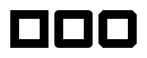
The left-hand square uses a MITER join that creates a sharp corner (the default if you don't specify a style). The middle square uses a ROUND join that rounds the corners off. The right-hand square uses a BEVEL join that cuts the corners off with a straight line.

This is largely a matter of preference. Use whichever you think looks best. If several lines or corners join at the same point, it is often a good idea to use the ROUND style, as it can look neater.

Mitre limit

When using the mitre style, if the two lines meet at a very small angle, the joint can get very long and look quite odd. To avoid this, pycairo applies a mitre limit. When the angle drops below a certain size, the MITER style automatically switches to BEVEL to prevent this. You don't need to worry about this. It happens automatically and is almost always a good thing.

You can change this behaviour using the miter_limit parameter of the stroke method. We won't cover it in detail here because it is quite a specialised function. Refer to the official Pycairo documentation for more details.

Line caps

We can also draw straight lines, using Line objects:

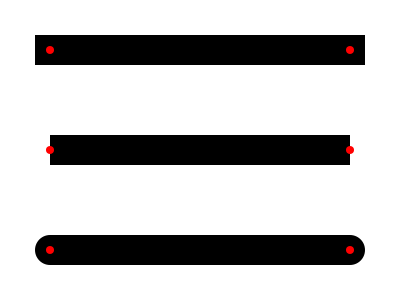
A line is defined by two points - the start of the line and the end of the line. When we stroke a line, we draw a line of the chosen colour and width from the start point to the endpoint.

We can choose the style of the line caps (ie the line ends) using the optional cap parameter of the stroke method:

• SQUARE, the top line above, squares off the line ends. The two red dots indicate the line endpoints. When you select square caps, the marked area extends slightly beyond the line's endpoints by a distance equal to half the line width. Square is the default cap type.
• BUTT, the middle line above, looks quite similar to the square case. The difference is that the line ends exactly on the endpoints, rather than extending beyond them.
• ROUND, the bottom line above, creates a rounded line end. The line end is a semicircle with a radius equal to half the line width.

Line caps only apply to the ends of lines, whereas line joins apply to the corners of shapes. Shapes such as rectangles or squares don't have ends, so the line cap parameter doesn't affect them. Lines have no corners, so the line join parameter does not affect them. Note that if two lines meet at a point, that doesn't mean they are joined, so the cap value controls the appearance rather than the join value.

Here is the code to draw the diagram above:

from generativepy.color import Color
from generativepy.drawing import make_image, setup
from generativepy.geometry import Line, Circle, ROUND, SQUARE, BUTT

def draw(ctx, width, height, frame_no, frame_count):
    setup(ctx, width, height, background=Color(1))

    (Line(ctx).of_start_end((50, 50), (350, 50))
              .stroke(Color("black"), 30, cap=SQUARE))
    Circle(ctx).of_center_radius((50, 50), 4).fill(Color("red"))
    Circle(ctx).of_center_radius((350, 50), 4).fill(Color("red"))

    (Line(ctx).of_start_end((50, 150), (350, 150))
              .stroke(Color("black"), 30, cap=BUTT))
    Circle(ctx).of_center_radius((50, 150), 4).fill(Color("red"))
    Circle(ctx).of_center_radius((350, 150), 4).fill(Color("red"))

    (Line(ctx).of_start_end((50, 250), (350, 250))
              .stroke(Color("black"), 30, cap=ROUND))
    Circle(ctx).of_center_radius((50, 250), 4).fill(Color("red"))
    Circle(ctx).of_center_radius((350, 250), 4).fill(Color("red"))

make_image("line-cap.png", draw, 400, 300)

This includes the three lines and the red circles that indicate the line ends.

Dash patterns

It is often useful to create dashed or dotted lines on a diagram. We can do this using the dash parameter of the stroke method. Here are some examples:

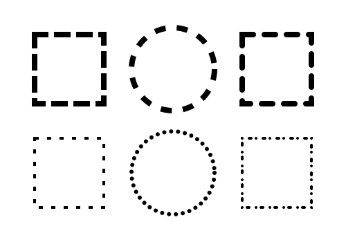
The dash pattern is specified by a list of values that define the on and off lengths of the dashed line, in user units (pixels by default).

Looking at the top row of shapes, each has a dash pattern of [16]. This means that the line will be solid for 16 pixels, then a gap of 16 pixels, repeated around the whole shape. However, each dash also includes line caps, as described above.

The square at the top left has the default line cap SQUARE. This means that, although the lines and gaps each have a nominal length of 16 pixels, the square line cap extends the lines. Since the line width is 8, this means that a cap of length 4 is added to each end of every line section. This means that each line has a marked length of 24 pixels. This means each gap is only 8 pixels (because the line occupies part of the gap).

The circle in the top centre uses the same measurements but has a BUTT style. This means each line finishes exactly at its nominal width, so the lines and gaps have equal lengths. This shape also shows how dashed lines follow curves.

The square at the top right has the same measurements but with a ROUND cap. It looks very similar to the square on the left, except that the dashes have rounded ends rather than square ends.

The bottom row of shapes demonstrates some other effects. The square on the left uses BUTT line caps, with a short length and a longer gap, to give a light dashed line. The circle is quite interesting: the line length is 0, but because the cap style is ROUND, the lines appear as circles (2 semicircular ends joined together), creating a dotted line. The square on the bottom right has a pattern of [0, 10, 3, 7], so it gives a dot-dash pattern.

Dash patterns can be used on any line, as we will see later. For example, you can outline text with dashed lines, and you can also apply dashes to line plots on graphs.

Here is the code for the examples above:

from generativepy.color import Color
from generativepy.drawing import make_image, setup
from generativepy.geometry import Rectangle, Circle, Square, BUTT, ROUND

def draw(ctx, width, height, frame_no, frame_count):
    setup(ctx, width, height, background=Color(1))

    (Square(ctx).of_corner_size((50, 50), 100)
                .stroke(Color("black"), 8, dash=[16]))
    (Circle(ctx).of_center_radius((250, 100), 60)
                .stroke(Color("black"), 8, dash=[16], cap=BUTT))
    (Square(ctx).of_corner_size((350, 50), 100)
                .stroke(Color("black"), 8, dash=[16], cap=ROUND))
    (Square(ctx).of_corner_size((50, 200), 100)
                .stroke(Color("black"), 4, dash=[6, 12], cap=BUTT))
    (Circle(ctx).of_center_radius((250, 250), 60)
                .stroke(Color("black"), 6, dash=[0, 10], cap=ROUND))
    (Square(ctx).of_corner_size((350, 200), 100)
                .stroke(Color("black"), 4, dash=[0, 10, 3, 7], cap=ROUND))

make_image("dash.png", draw, 500, 350)

Other features of the setup function

Looking back at our first example code:

from generativepy.color import Color
from generativepy.drawing import setup, make_image
from generativepy.geometry import Rectangle

def draw(ctx, width, height, frame_no, frame_count):
    setup(ctx, width, height, background=Color("grey"))
    Rectangle(ctx).of_corner_size((100, 150), 250, 200).fill(Color("orange"))

make_image("rectangle.png", draw, 500, 400)

This creates a 500-by-400-pixel image. Now suppose we decided that we actually needed the image to be 1000 by 800 pixels, that is twice as big. We can do this quite easily by altering the size in the make_image call. But the problem then is that the rectangle size in the draw function is also wrong. That would need adjusting. We can do that easily, but what if the drawing function was very complex - we would need to go through and alter the entire drawing code.

The setup function provides an easy solution. Consider the following code:

from generativepy.color import Color
from generativepy.drawing import setup, make_image
from generativepy.geometry import Rectangle

def draw(ctx, width, height, frame_no, frame_count):
    setup(ctx, width, height, width=500, background=Color("grey"))
    Rectangle(ctx).of_corner_size((100, 150), 250, 200).fill(Color("orange"))

make_image("rectangle.png", draw, 1000, 800)

Here, we have changed the image size to 1000 by 800 in the make_image call, but we have added an extra parameter width=500 in the setup call.

This tells setup to scale the drawing canvas. Since the page width is 1000 and the setup width parameter is 500, setup introduces a scale factor of 2. So everything we draw appears twice as big, which is exactly what we want. And since it is a vector drawing, the scale is done smoothly, without any pixelation.

setup also has a height parameter. We can use that instead of width. If we set height to 400, since the pixel height in make_image is 800, we would get a scale factor of 2. You can set either the width or height, whichever is more convenient. Either way, it decouples the pixel size of the image from the dimensions you use in the drawing code. So you can write your drawing code without committing to the final image size.

The scale factor doesn't have to be an integer. For example, if you discovered that your 1000 pixel image really needed to be 2100 pixels wide, you could do that. This would be a scale factor of 2.1, but because it's a vector image, it would still render perfectly.

You would normally only specify either width or height. If you specify both, the image might be scaled by a different amount in each direction. It would still render cleanly, but shapes would be distorted (for example, squares would be stretched into rectangles). That isn't normally what you would want, but it can be useful in some cases.

setup also has a flip parameter that flips the axes in the y direction, so y coordinate values start from 0 at the bottom of the image. This can be useful if you prefer a graph-like coordinate system when designing an image. It also has startx and starty, which shift the image on the page. This can be useful for adding a border to an image.

setupis provided as a convenience. You can also change the image coordinates and scale using Transform objects, as described in a later tutorial.

Other shapes

generativepy supports several other shapes:

• More polygons
  • Triangles
  • General polygons
  • Regular polygons
• Line variants - segment, ray, or infinite line
• Circle variants
  • Sector, segment, and arc of a circle
  • Ellipses

More polygons

This code draws several other types of polygons:

from generativepy.color import Color
from generativepy.drawing import make_image, setup
from generativepy.geometry import (Triangle, FillParameters, StrokeParameters,
                                   Polygon, RegularPolygon, ROUND)


def draw(ctx, width, height, frame_no, frame_count):
    setup(ctx, width, height, background=Color(1))

    f = FillParameters(Color("powderblue"))
    s = StrokeParameters(Color("darkslateblue"), 6, dash=[10, 8],
                         cap=ROUND, join=ROUND)

    Triangle(ctx).of_corners((50, 150), (200, 120), (100, 50)).fill(f).stroke(s)

    points = ((300, 50), (350, 100), (330, 200), (270, 200), (250, 100))
    Polygon(ctx).of_points(points).fill(f).stroke(s)

    points = ((500, 50), (550, 100), (530, 200), (470, 200), (450, 100))
    Polygon(ctx).of_points(points).open().stroke(s)

    p = RegularPolygon(ctx).of_centre_sides_radius((150, 300), 8, 70).stroke(s)
    print(p.inner_radius)

make_image("more-polygons.png", draw, 600, 400)

Here is the result:

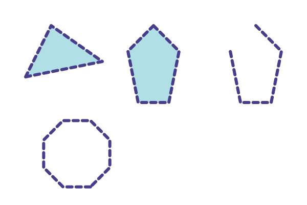
First, you will notice that we have defined a couple of extra items:

• A FillParameters object f, initialised with a colour.
• A StrokeParameters object s, initialised with a colour, thickness, plus dash, cap, and join values.

We can use f and s as parameters for the fill and stroke methods of any object. This is useful if we want to draw several objects in the same style because it saves repetition.

The top left shape is a Triangle. This has an of_corners method to define its three corners, as (x, y) tuples. It is then filled and stroked as usual, using f and s to control the style.

The top centre shape is a Polygon. This has an of_points method to define its vertices. The vertices are provided as a sequence of (x, y) tuples.

The top right shape is another Polygon. This time, it has an extra call to its open method, which creates an open polygon, meaning the final vertex is not connected to the first vertex. This is sometimes called a polyline because you can think of it as a set of connected lines rather than a shape. We haven't filled this shape, but you can if you wish. That would fill the shape as if it were a closed polygon, but of course, the outline would still be open.

The bottom left is a RegularPolygon. We call of_centre_sides_radius passing in:

• The position of the centre of the polygon, as an (x, y) tuple.
• The required number of sides. We passed in 8 to create an octagon.
• The radius of the shape. This controls the polygon's size. It is the distance from the centre to any vertex of the polygon.

By default, the polygon is drawn with the bottom edge horizontal (as shown). The of_centre_sides_radius function has an optional angle parameter that rotates the shape clockwise by the supplied angle, specified in radians.

A RegularPolygon has a few useful properties, calculated from the parameters:

• side_len - the length of a side of the polygon
• interior_angle - the interior angle of the polygon (in radians)
• exterior_angle - the exterior angle of the polygon (in radians)
• inner_radius - the inner radius (distance from the centre to the midpoint of any side)
• outer_radius - the outer radius of the polygon (this is just the radius we supplied)
• vertices - a list of the vertices as (x, y) tuples

Line Variants

We have seen how to draw a line using the Line class. This draws a straight line between two points, which here we will call p1 and p2.

In computer graphics, a line normally means a finite line between two points. But in mathematics, we define three different types of lines:

• A line segment has finite length. It starts at p1 and ends at p2.
• A ray has semi-infinite length. It starts at p1 and passes through p2, but it extends beyond p2 right off to infinity. A ray is sometimes called a half-line.
• A line has infinite length. It passes through p1 and p2, but it extends to infinity in both directions.

By default, Line draws a line segment, but it can also draw rays and (infinite) lines. Here is some example code:

from generativepy.color import Color
from generativepy.drawing import make_image, setup
from generativepy.geometry import StrokeParameters, Circle, Line, ROUND

def draw(ctx, width, height, frame_no, frame_count):
    setup(ctx, width, height, background=Color(1))

    def dot(p):
        Circle(ctx).of_center_radius(p, 8).fill(Color("red"))

    s = StrokeParameters(Color("darkgreen"), 6, cap=ROUND)

    p1 = (100, 300)
    p2 = (150, 100)
    Line(ctx).of_start_end(p1, p2).as_segment().stroke(s)
    dot(p1)
    dot(p2)

    p1 = (200, 300)
    p2 = (250, 100)
    Line(ctx).of_start_end(p1, p2).as_ray().stroke(s)
    dot(p1)
    dot(p2)

    p1 = (300, 300)
    p2 = (350, 100)
    Line(ctx).of_start_end(p1, p2).as_line().stroke(s)
    dot(p1)
    dot(p2)

make_image("more-lines.png", draw, 500, 400)

Here is the result:

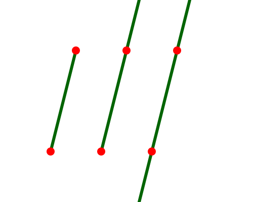
In the code, we have created a dot function that draws a small red circle to mark a point.

The line on the left of the image is a segment. It just extends from one point to the other. The code includes a call to as_segment, although it isn't really needed because a segment is the default. The line in the centre is a ray that extends from the first point, through the second point, and then disappears off the edge of the image. The line on the right is an infinite line that passes through both points and disappears off the edge of the image in both directions.

One thing to bear in mind is that the Line class doesn't actually draw an infinite line. It just draws a very long line that goes beyond the edge of the image. If you create a very large image, you might need to make the line longer. The as_line and as_ray methods accept an optional parameter infinity that you can set to a suitable large number if needed.

Circle variants

We have already seen how to draw a circle, but generativepy offers some variants:

• A sector of a circle is like a pie slice taken out of the circle
• A segment is part of a circle cut off by a chord (a chord is a straight line between two points on the circumference)
• An arc is part of the circumference.

It is also possible to draw an ellipse, which is also covered in this section.

Here is the code to draw these shapes:

import math

from generativepy.color import Color
from generativepy.drawing import make_image, setup
from generativepy.geometry import Circle, FillParameters, StrokeParameters

def draw(ctx, width, height, frame_no, frame_count):
    setup(ctx, width, height, background=Color(1))

    f = FillParameters(Color("yellow"))
    s = StrokeParameters(Color("black"), 6)

    (Circle(ctx).of_center_radius((150, 150), 75)
                .fill(f).stroke(s))
    (Circle(ctx).of_center_radius((350, 150), 75)
                .as_sector(math.radians(0), math.radians(135))
                .fill(f).stroke(s))
    (Circle(ctx).of_center_radius((150, 350), 75)
                .as_segment(math.radians(-90), math.radians(20))
                .fill(f).stroke(s))
    (Circle(ctx).of_center_radius((350, 350), 75)
                .as_arc(math.radians(-90), math.radians(20))
                .stroke(s))

make_image("more-circles.png", draw, 500, 500)

Here is the result:

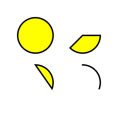
The top left shape is a normal circle. The other shapes are described below.

Sectors

The top right shape is a sector, created with this code:

    (Circle(ctx).of_center_radius((350, 150), 75)
                .as_sector(math.radians(0), math.radians(135))
                .fill(f).stroke(s))

Here, we declare a circle as usual. But there is an extra call to as_sector. This creates a sector using the supplied angles of 0° and 135°. This requires a bit more explanation. First, generativepy measures angles clockwise from the positive x-axis. This is illustrated here:

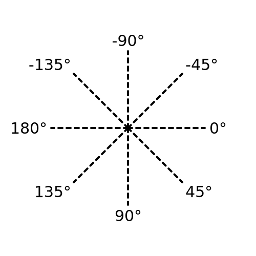
This differs from the standard mathematical convention, but it is common in computer graphics because we usually measure the y-direction downward from the top of the image. Notice that angles above the horizontal are negative.

generativepy measures angles in radians. However, if you prefer to work in degrees, you can use the math.radians function to convert degrees to radians, as shown in the example code.

Finally, the sector is defined as the part of the circle created when we move clockwise from the first angle to the second angle. This is shown here:

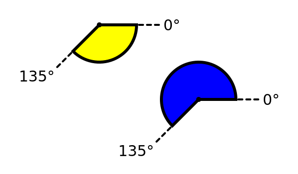
The yellow shape shows how the sector is created from a circle by taking the part of the circle between 0° and 135° clockwise. To draw the blue sector, we would take the part of the circle between 135° and 0° clockwise. We would need to swap the start and end angles in the as_sector call, like this:

    (Circle(ctx).of_center_radius((350, 150), 75)
                .as_sector(math.radians(135), math.radians(0))
                .fill(f).stroke(s))

Segments

The bottom left of the original diagram shows a segment. This is formed from part of a circle by taking two points on the circumference and drawing a straight line between them (unlike a sector where we draw lines back to the centre of the circle):

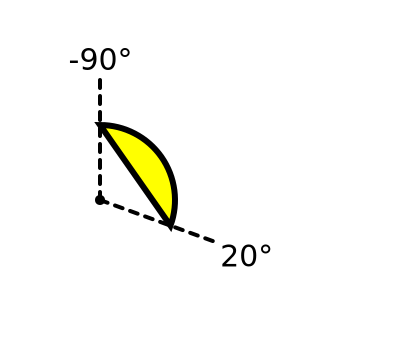
We draw a segment by adding an as_segment call to the circle code, like this:

    (Circle(ctx).of_center_radius((150, 350), 75)
                .as_segment(math.radians(-90), math.radians(20))
                .fill(f).stroke(s))

This time the segment is formed from the part of the circle starting at -90° and moving clockwise to 20°. Again we can draw the opposite segment by swapping the angles.

Arcs

An arc is part of the circumference of a circle. It is a line, rather than a two-dimensional shape. It appears in the bottom right of the original diagram. We create an arc like this:

    (Circle(ctx).of_center_radius((350, 350), 75)
                .as_arc(math.radians(-90), math.radians(20))
                .stroke(s))

An arc is created in the same way as a segment. We call as_arc rather than as_segment. The only difference is that an arc doesn't include the extra line joining the two points on the circumference.

Since an arc is just a line, you would not normally fill it.

Ellipses

An ellipse is like a circle that has been stretched in one direction. Here are a couple of examples:

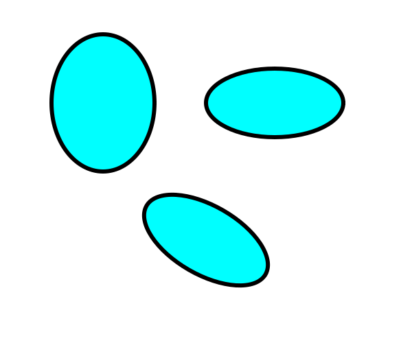
We draw an ellipse using the Ellipse class, like this:

import math

from generativepy.color import Color
from generativepy.drawing import make_image, setup
from generativepy.geometry import (FillParameters, StrokeParameters,
                                   Ellipse, Transform)


def draw(ctx, width, height, frame_no, frame_count):
    setup(ctx, width, height, background=Color(1))

    f = FillParameters(Color("cyan"))
    s = StrokeParameters(Color("black"), 6)

    (Ellipse(ctx).of_center_radius((150, 150), 75, 100)
                .fill(f).stroke(s))
    (Ellipse(ctx).of_center_radius((400, 150), 100, 50)
                .fill(f).stroke(s))
    Transform(ctx).translate(300, 350).rotate(math.radians(30))
    (Ellipse(ctx).of_center_radius((0, 0), 100, 50)
                .fill(f).stroke(s))

make_image("ellipse.png", draw, 600, 500)

The Ellipse class is very similar to the Circle class, except that its of_center_radius method accepts an x-radius and a y-radius. In the top left example above, the x-radius is smaller than the y-radius, so the ellipse is taller than it is wide. In the top right example, the x-radius is larger than the y-radius, so the ellipse is wider than it is tall.

We can also create segments, sectors, and arcs of an ellipse in the same way as we do for circles.

The ellipse class only allows us to create ellipses where the two axes are aligned with the x and y directions. To create an ellipse with axes at an angle, we need to transform the drawing space. The bottom, centre example shows this: we use Transform to rotate the drawing space by 30° before drawing the ellipse. We will cover Transform in a later chapter.

Related articles

• Introduction to generativepy
• Color in generativepy
• Graphs in generativepy
• Advanced graphing features in generativepy