Travelling salesman problem

The travelling salesman problem (often abbreviated to TSP) is a classic problem in graph theory. It has many applications, in many fields. It also has quite a few different solutions.

The problem

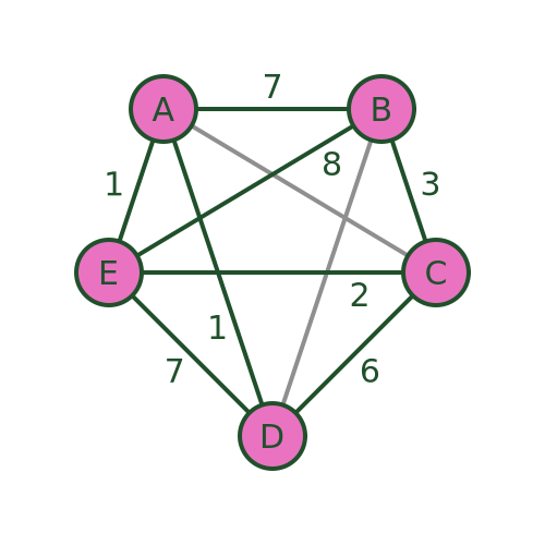
The problem is usually stated in terms of a salesman who needs to visit several towns before eventually returning to the starting point. There are various routes he could take, visiting the different towns in different orders. Here is an example:

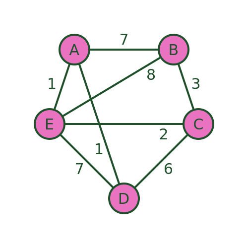
There are several different routes that will visit every town. For example, we could visit the towns in the order A, B, C, D, E, then back to A. Or we could use the route A, D, C, E, B then back to A.

But not all routes are possible. For example, we cannot use a route A, D, E, B, C and then back to A, because there is no road from C to A.

The aim is to find the route that visits all the towns with the minimum cost. The cost is shown as the weight of each edge in the graph. This might be the distance between the towns, or it might be some other measure. For example, it might be the time taken to travel between the towns, which might not be proportionate to the distance because some roads have lower speed limits or are more congested. Or, if the salesman was travelling by train, it might be the price of the tickets.

The salesman can decide to optimise for whatever measure he considers to be most important.

Alternative applications and variants

TSP applies to any problem that involves visiting various places in sequence. One example is a warehouse, where various items need to be fetched from different parts of a warehouse to collect the items for an order. In the simplest case, where one person fetches all the items for a single order and then packs and dispatches the items, a TSP algorithm can be used. Of course, a different route would be required for each order, which would be generated by the ordering system.

Another interesting example is printed circuit board (PCB) drilling. A PCB is the circuit board you will find inside any computer or other electronic device. They often need holes drilled in them, including mounting holes where the board is attached to the case and holes where component wires need to pass through the board. These holes are usually drilled by a robot drill that moves across the board to drill each hole in the correct place. TSP can be used to calculate the optimum drilling order.

The TSP algorithm can be applied to directed graphs (where the distance from A to B might be different to the distance from B to A). Directed graphs can represent things like one-way streets (where the distance might not be the same in both directions) or flight costs (where the price of a single airline ticket might not be the same in both directions).

There are some variants of the TSP scenario. The mTSP problem covers the situation where there are several salesmen and exactly one salesman must visit each city. This applies to delivery vans, where there might be several delivery vans. The problem is to decide which parcels to place on each van and also to decide the route of each van.

The travelling purchaser problem is another variant. In that case, a purchaser needs to buy several items that are being sold in different places, potentially at different prices. The task is to purchase all the items, minimising the total cost (the cost of the items and the cost of travel). A simple approach would be to buy each item from the place where it is cheapest, in which case this becomes a simple TSP. However, it is not always worth buying every item from the cheapest place because sometimes the travel cost might outweigh the price difference.

In this article, we will only look at the basic TSP case.

Brute force algorithm

We will look at 3 potential algorithms here. There are many others. The first, and simplest, is the brute force approach.

We will assume that we start at vertex A. Since we intend to make a tour of the vertices (ie visit every vertex once and return to the original vertex) it doesn't matter which vertex we start at, the shortest loop will still be the same.

So we will start at A, visit nodes B, C, D, and E in some particular order, then return to A.

To find the shortest route, we will try every possible ordering of vertices B, C, D, E, and record the cost of each one. Then we can find the shortest.

For example, the ordering ABCDEA has a total cost of 7+3+6+7+1 = 24.

The ordering ABCEDA (i.e. swapping D and E) has a total cost of 7+3+2+7+1 = 20.

Some routes, such as ADEBCA are impossible because a required road doesn't exist. We can just ignore those routes.

After evaluating every possible route, we are certain to find the shortest route (or routes, as several different routes may happen to have the same length that also happens to be the shortest length). In this case, the shortest route is AECBDA with a total length of 1+8+3+6+1 = 19.

The main problem with this algorithm is that it is very inefficient. In this example, since we have already decided that A is the start/end point, we must work out the visiting order for the 4 towns BCDE. We have 4 choices of the first town, 3 choices for the second town, 2 choices for the third town, and 1 choice for the fourth town. So there are 4! (factorial) combinations. That is only 24 combinations, which is no problem, you could even do it by hand.

If we had 10 towns (in addition to the home town) there would be 10! combinations, which is 3628800. Far too many to do by hand, but a modern PC might be able to do that in a fraction of a second if the algorithm was implemented efficiently.

If we had 20 towns, then the number of combinations would be of order 10 to the power 18. If we assume a computer that could evaluate a billion routes per second (which a typical PC would struggle to do, at least at the time of writing), that would take a billion seconds, which is several decades.

Of course, there are more powerful computers available, and maybe quantum computing will come into play soon, but that is only 20 towns. If we had 100 towns, the number of combinations would be around 10 to the power 157, and 1000 towns 10 to the power 2568. For some applications, it would be quite normal to have hundreds of vertices. The brute force method is impractical for all but the most trivial scenarios.

Nearest neighbour algorithm

The nearest neighbour algorithm is what we might call a naive attempt to find a good route with very little computation. The algorithm is quite simple and obvious, and it might seem like a good idea to someone who hasn't put very much thought into it. You start by visiting whichever town is closest to the starting point. Then each time you want to visit the next town, you look at the map and pick the closest town to wherever you happen to be (of course, you will ignore any towns that you have visited already). What could possibly go wrong?

Starting at A, we visit the nearest town that we haven't visited yet. In this case D and E are both distance 1 from A. We will (completely arbitrarily) always prioritise the connections in alphabetical order. So we pick D.

As an aside, if we had picked E instead we would get a different result. It might be better, but it is just as likely to be worse, so there is no reason to chose one over the other.

From D, the closest town is C with a distance of 6 (we can't pick A because we have already been there).

From C the closest town is E with distance 2. From E we have to go to B because we have already visited every other town - that is a distance of 8. And from B we must return to A with a distance of 7.

The final path is ADCEBA and the total distance is 1+6+2+8+7 = 24.

The path isn't the best, but it isn't terrible. This algorithm will often find a reasonable path, particularly if there is a natural shortest path. However, it can sometimes go badly wrong.

The basic problem is that the algorithm doesn't take account of the big picture. It just blindly stumbles from one town to whichever next town is closest.

In particular, the algorithm implicitly decides that the final step will be B to A. It does this based on the other distances, but without taking the distance BA into account. But what if, for example, there is a big lake between B and A that you have to drive all the way around? This might make the driving distance BA very large. A more sensible algorithm would avoid that road at all costs, but the nearest neighbour algorithm just blindly leads us there.

We can see this with this revised graph where BA has a distance of 50:

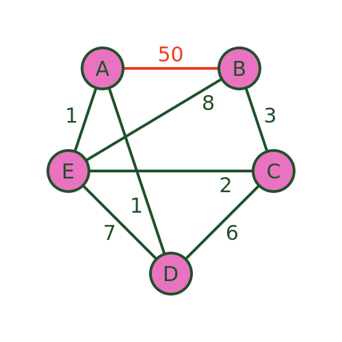
The algorithm will still recommend the same path because it never takes the distance BA into account. The path is still ADCEBA but the total distance is now 1+6+2+8+50 = 67. There are much better routes that avoid BA.

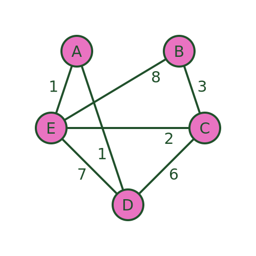
An even worse problem can occur if there is no road at all from B to A. The algorithm would still guide us to town B as the final visit. But in that case, it is impossible to get from B to A to complete the journey:

Bellman–Held–Karp algorithm

The Bellman–Held–Karp algorithm is a dynamic programming algorithm for solving TSP more efficiently than brute force. It is sometimes called the Held–Karp algorithm because it was discovered by Michael Held and Richard Karp, but it was also discovered independently by Richard Bellman at about the same time.

The algorithm assumes a complete graph (ie a graph where every vertex is connected to every other). However, it can be used with an incomplete graph like the one we have been using. To do this, we simply add extra the missing connections (shown below in grey) and assign them a very large distance (for example 1000). This ensures that the missing connections will never form part of the shortest path:

The technique works by incrementally calculating the shortest path for every possible set of 3 towns (starting from A), then for every possible set of 4 towns, and so on until it eventually calculates the shortest path that goes from A via every other town and back to A.

Because the algorithm stores its intermediate calculations and discards non-optimal paths as early as possible, it is much more efficient than brute force.

Step 1

We will use the following notation. We will use this to indicate the distance between towns A and B:

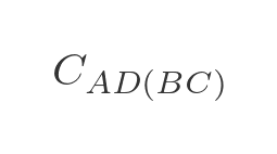
And we will use this to indicate the cost (ie the total distance) from A to C via B:

Here are some examples:

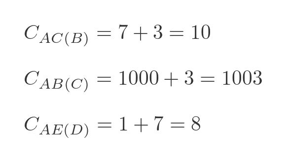
The first example is calculated by adding the distance AB to BC, which gives 10. The second example is calculated by adding AC to CB. But since there is no road from A to C, we give that a large dummy distance of 1000, so that total cost is 1003, which means it is never going to form a part of the shortest route. The third example is calculated by adding the distance AD to DE, which gives 8.

In the first step, we will calculate the value of every possible combination of 2 towns starting from A. There are 12 combinations: AB(C), AB(D), AB(E), AC(B), AC(D), AC(E), AD(B), AD(C), AD(E), AE(B), AE(C), AE(D).

These values will be stored for later use.

Step 2

For step 2 we need to extend our notation slightly. We will use this to indicate the lowest cost from A to D via B and C (in either order):

To be clear, this could represent one of two paths - ABCD or ACBD whichever is shorter. We can express this as a minimum of two values:

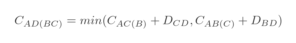
This represents the 2 ways to get from A to D via B and C:

• We can travel from A to C via B, and then from C to D.
• We can travel from A to B via C, and then from B to D.

We have already calculated A to C via B (and all the other combinations) in step 1, so all we need to do is add the values and find the smallest. In this case:

• A to C via B is 10, C to D is 6, so the total is 16.
• A to B via C is 1003, B to D is 1000, so the total is 2003.

Clearly, ABCD is the best route.

We need to repeat this for every possible combination of travelling from A to x via y and z. There are, again, 12 combinations: AB(CD), AB(CE), AB(DE), AC(BD), AC(BE), AC(DE), AD(BC), AD(BE), AD(CE), AE(BC), AE(BD), AE(CD).

We store these values, along with the optimal path, for later use.

Step 3

In the next step, we calculate the optimal route for travelling from A to any other town via 3 intermediate towns. For example, travelling from A to E via B, C, and D (in the optimal order) is written as:

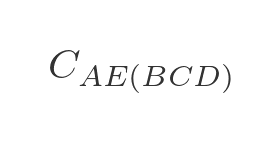
There are 3 paths to do this:

• A to D via B and C, then from D to E.
• A to C via B and D, then from C to E.
• A to B via C and D, then from B to E.

We will choose the shortest of these three paths:

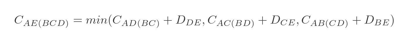
Again we have already calculated all the optimal intermediate paths. This time there are only 4 combinations we need to calculate: AB(CDE), AC(BDE), AD(BCE), and AE(BCD).

Final step

We are now in a position to calculate the optimal route for travelling from A back to A via all 4 other towns:

We need to evaluate each of the 4 options in step 3, adding on the extra distance to get back to A:

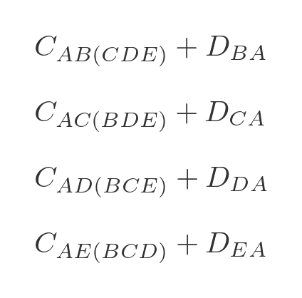
We can then choose the option that has the lowest total cost, and that will be the optimal route.

Performance

The performance of the Bellman–Held–Karp algorithm can be expressed in big-O notations as:

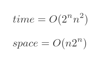
The time performance is approximately exponential. As the number of towns increases, the time taken will go up exponentially - each time an extra town is added, the time taken will double. We are ignoring the term in n squared because the exponential term is the most significant part.

Exponential growth is still quite bad, but it is far better than the factorial growth of the brute-force algorithm.

It is also important to notice that the algorithm requires memory to store the intermediate results, which also goes up approximately exponentially. The brute force algorithm doesn't have any significant memory requirements. However, that is usually an acceptable trade-off for a much better time performance.

The stages above describe how the algorithm works at a high level. We haven't gone into great detail about exactly how the algorithm keeps track of the various stages. Over the years since its discovery, a lot of work has been put into optimising the implementation. Optimising the implementation won't change the time complexity, which will still be roughly exponential. However, it might make the algorithm run several times faster than a poor implementation.

We won't cover this in detail, but if you ever need to use this algorithm for a serious purpose, it is worth considering using an existing, well-optimised implementation rather than trying to write it yourself. Unless you are just doing it for fun!

Other algorithms

Even the Bellman–Held–Karp algorithm has poor performance for modestly large numbers of towns. 100 towns, for example, would be well beyond the capabilities of a modern PC.

There are various heuristic algorithms that are capable of finding a good solution, but not necessarily the best possible solution, in a reasonable amount of time. I hope to cover these in a future article.

See also

• Graphs
• Adjacency matrices
• The seven bridges of Königsberg
• Dijkstra's algorithm