Dijkstra's algorithm

Here is a weighted graph showing the connections between a set of vertices:

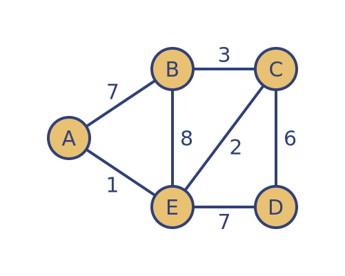
In a weighted graph, each connection (or edge) between two vertices has a weight associated with it. This weight can be used to represent various things. For example, if the vertices represent towns, the weight could represent the distance between the towns, or it might represent the cost of a train ticket between the towns, or the time it would take to cycle between the towns, etc. As a concrete example, in this article, we will assume the weights represent distance, but the calculations are the same no matter what they represent.

It is often useful to know the shortest route between 2 towns, and for a complex network, it might not be obvious which route is the best. Dijkstra's algorithm provides a simple, efficient method to determine the shortest route between 2 vertices.

Dijkstra's algorithm

Dijkstra's algorithm works by first selecting a fixed starting point, called the source vertex, and then calculating the shortest distance of every other vertex from the source vertex.

The algorithm assumes that the weights are all positive because it assumes that the distance from X to Y to Z is always greater than the distance from X to Y. This will always be true for distances. If you have a graph with negative or zero weights, Dijkstra's algorithm cannot be used.

The algorithm also assumes that the graph is connected (ie it is possible to find a path between any two vertices X and Y), that the graph is undirected (the distance from X to Y is always the same as the distance from Y to X), and that it is not a multigraph (there cannot be more than 1 direct connection between any X and Y), and it doesn't contain any loops (X is not connected to itself).

The result will be a tree that shows the shortest route between the source vertex and every other vertex. A tree is a graph that contains no cycles, in other words, there is one and only one path between any 2 vertices X and Y. Here is the solution for the graph above, assuming the source vertex is A:

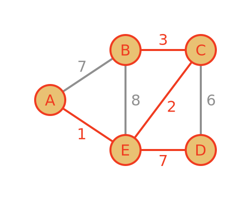
The shortest path from A to any other vertex follows the red path.

Algorithm - setup

The algorithm operates step by step, one vertex at a time, starting with the source vertex A. Initially, we will grey out all the vertices to indicate that we do not yet know the shortest distance between any of the vertices:

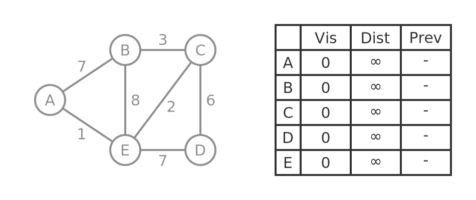
The table holds values for each vertex:

• Visited - we say a vertex has been visited when we know its shortest path from A. We will visit the vertices one by one.
• Distance - the shortest path from this vertex to the source vertex. Initially, we set this to infinity, the value will be filled with a tentative distance that might change as the algorithm progresses. Once a vertex has been visited, its true shortest distance will be known.
• Previous - the previous vertex in the shortest path. This allows us to reconstruct the shortest path once the algorithm is complete.

Algorithm - step 1

The algorithm starts with the source vertex, which is A in our example. At this point, we know that the distance from A to A is 0, of course. As above, we say we have visited vertex A, because we know the distance from A to A.

From this starting point, we look at all the neighbours of A (the vertices that can be reached in a single step). The neighbours are B and E.

The tentative shortest distance from A to its neighbour B is 7 (assuming we go from A directly to B) but at this stage that value might prove to be incorrect. We say we have accessed B, but we haven't visited B yet.

Similarly, the tentative distance from A to E is 1, but again that might change, and again we have accessed E but not visited it.

Here is the graph with visited vertices in red, accessed vertices in blue, and all the other vertices in grey:

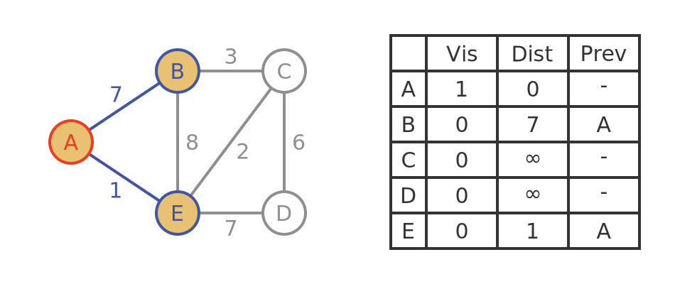
The table has been updated to show that we have visited A. It also shows that our tentative distance to B is 7, with A as the previous vertex. In addition, our tentative distance to E is 1, with A as the previous vertex.

Algorithm - step 2

In the next step, we look at all the unvisited vertices and choose the one with the smallest tentative distance as the starting point for the next step. From the previous table, this is E with a distance of 1 (since B has a distance of 7 and the others are infinity).

This next fact is absolutely key to the algorithm: we now KNOW that the shortest distance from A to E is 1.

How do we know that? Well, we specifically selected E because it has the smallest tentative distance. To get from A to E we can either go direct, or we can go via B in some way. For example, we could go ABE, or maybe ABCE. But here is the thing, the distance from A to B is greater than the distance from A to E, so any route that goes via B must be longer than A to E. Therefore AE must be the shortest route from A to E.

So we can mark vertex E as visited because we know its true distance.

Notice that we don't yet know the shortest route from A to B. It might be AB, with a distance of 8. But since the distance AE is only 1, there might be a shorter route to B via E. At this point (based on the parts of the graph we have analysed so far) we simply don't know. That is why we call the distance tentative.

Now, once again, we must look at the unvisited neighbours of the newly visited vertex E. The neighbours are B, C and D.

For each neighbour, we find its distance from the source vertex A via the current vertex E. If that distance is less than the current tentative distance, we update it.

For B, the distance AEB is 1 + 8 = 9. This is greater than the current tentative distance for B of 8, so we leave the current distance unchanged.

C has a tentative distance of infinity, so we replace it with the distance via E, which is AEC. This is 1 + 2 = 3. Similarly, the tentative distance of D is replaced with AED, which is 1 + 5 = 6

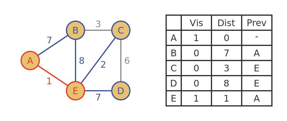
Here is the updated graph and table, with E marked as visited and the new distances added:

Algorithm - step 3

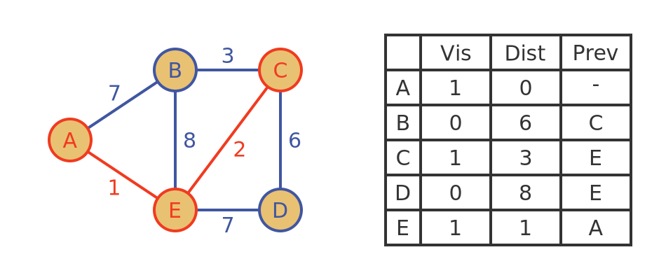
In the next step, we again look at all the unvisited vertices and choose the one with the smallest tentative distance to go forward for the next step. From the previous table, B, C and D are unvisited, and C has the smallest distance of 3, and a previous vertex E.

We mark C as visited.

Now we update all the unvisited neighbours of C, these are B and D.

The tentative distance of B, via C, is 3 + 3 = 6. This is calculated from the true distance of C, plus the weight of the edge BC, which are both equal to 3. Since this new distance is less than the previous distance for B (7), we set the distance of B to 6 and the previous vertex to C.

The tentative distance of D via C is 3 + 6 = 9. Since that is greater than the current distance, we leave it unchanged. Here is the updated graph:

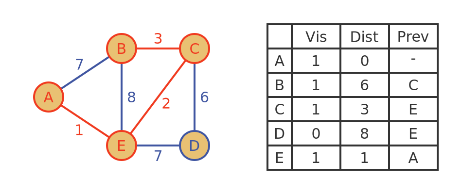
Algorithm - step 4

We are nearly finished! Only B and D are unvisited, and B has the shortest tentative distance, so we will mark it as visited with a true distance of 6.

B has no unvisited neighbours so there is nothing more to do in this step.

Algorithm - step 5

Now there is only one unvisited vertex, D, so we just make it as visited with a true distance of 8. Since there are no remaining unvisited vertices, we are done.

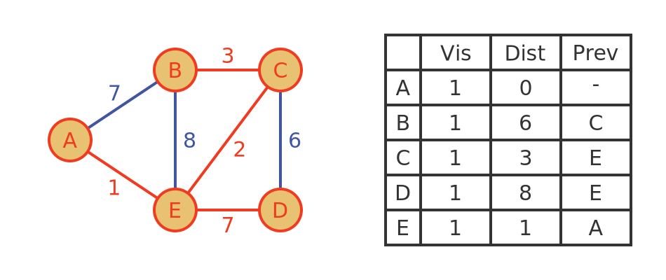
Algorithm - conclusion

The result of the algorithm is a tree that can be used to calculate the path and distance of any vertex from the source, A:

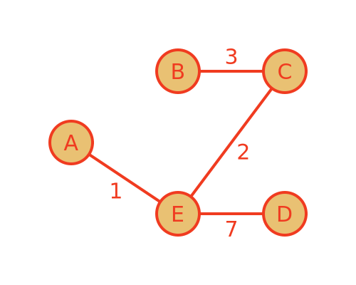
So, for example, the shortest path to D is AED with a length of 8. The shortest path to B is AECB with a length of 6.

It is important to remember that this tree is only valid for routes that start from A. If we start from a different vertex, the route might not be the shortest. For example, if we travel from C to D, according to this tree we have to go via E, with a total distance of 9. But looking at the full mgraph, we can see that going from C to D directly only has a distance of 6.

Python implementation of Dijkstra's algorithm

Here is a simple implementation of the algorithm in Python.

INFINITY = 1000
vertex_count = 5
start_vertex = 0
names = ("A", "B", "C", "D", "E")
graph = (
    #A  B  C  D  E
    (0, 7, 0, 0, 1,),  # A
    (7, 0, 3, 0, 8,),  # B
    (0, 3, 0, 6, 2,),  # C
    (0, 0, 6, 0, 7,),  # D
    (1, 8, 2, 7, 0,),  # E
)
visited = [0]*vertex_count
shortest_distance = [INFINITY] * vertex_count
previous = [""]*vertex_count

def get_unvisited_vertices():
    return [i for i in range(vertex_count) if not visited[i]]

def get_unvisited_neighbours(vertex):
    row = graph[vertex]
    return [i for i in range(vertex_count) if row[i] and not visited[i]]

def get_shortest_unvisited():
    shortest_unvisited = -1
    current_shortest_distance = INFINITY
    for vertex in get_unvisited_vertices():
        if shortest_distance[vertex] < current_shortest_distance:
            shortest_unvisited = vertex
            current_shortest_distance = shortest_distance[vertex]
    return shortest_unvisited


def calculate_distances():
    shortest_distance[start_vertex] = 0

    while not all(visited):
        current = get_shortest_unvisited()
        visited[current] = 1

        unvisited_neighbours = get_unvisited_neighbours(current)
        for vertex in unvisited_neighbours:
            if shortest_distance[current] + graph[current][vertex] < shortest_distance[vertex]:
                shortest_distance[vertex] = shortest_distance[current] + graph[current][vertex]
                previous[vertex] = names[current]
                visited[current] = 1

calculate_distances()
print(names)
print(shortest_distance)
print(previous)

To give a brief explanation, in the first section, we initialise all the data structures. A couple of points of note, we define INFINITY as 1000 - we can use any value that is larger than the largest weight on the graph, and since all the weights are single digits, 1000 is plenty large enough to be considered infinite.

In addition, we have used an adjacency matrix to define the graph. This is convenient for processing the graph in code.

We next define some simple utility functions, whose implementations are hopefully self-explanatory:

• get_unvisited_vertices() returns a list of the indices of every vertex that is currently not visited.
• get_unvisited_neighbours(vertex) returns a list of the indices of every vertex that is a neighbour of the supplied vertex and is currently not visited.
• get_shortest_unvisited() returns the index of the unvisited vertex that has the shortest tentative distance, or -1 if there are no remaining unvisited vertices.

Finally, the calculate_distances() function, first sets the shortest_distance of the source vertex to 0, and then it executes the main loop until all the vertices have been visited.

The main loop operates exactly as described above. It first finds the unvisited vertex with the shortest distance and marks it as visited. It then adjusts the tentative distances of all the other unvisited vertices.

See also

• Graphs
• Adjacency matrices
• The seven bridges of Königsberg
• Travelling salesman problem