2D transformation matrices - scaling, rotation, shear and translation

A matrix can be used to describe or calculate transformations in 2 dimensions. It can be used to describe any affine transformation. This includes scaling, rotating, translating, skewing, or any combination of those transformations.

Most 2D transformations can be represented by a 2 × 2 matrix. However, translation cannot be expressed this way, so a 3 × 3 matrix using homogeneous coordinates is required whenever translation is involved, as described below.

Applying a matrix transformation

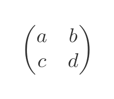
If we have a 2 ⨯ 2 matrix:

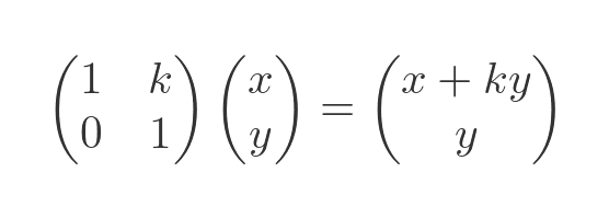
If we multiply this matrix by a column vector we get another column vector:

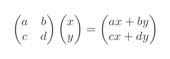
The elements of the new vector are formed from a linear combination of the elements of the original vector.

Notice that, by convention, the matrix comes before the vector in the multiplication.

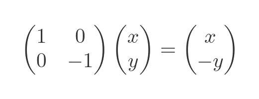
Scaling transformations

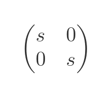
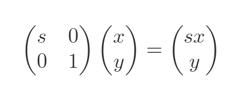
A scaling transformation uses the following matrix:

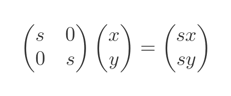
Here is the effect it has on a vector:

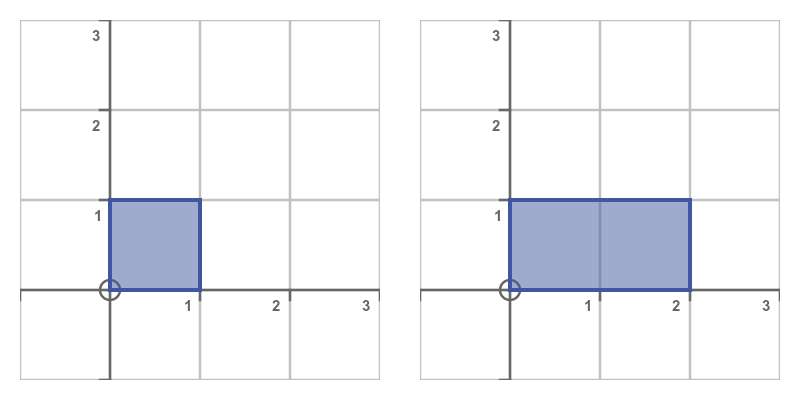
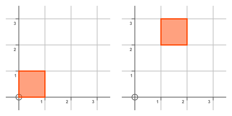
If we take a unit square and apply this transform to each of its vertices, we get the new shape on the right. We have used an s value of 2, which scales the shape by a factor of 2:

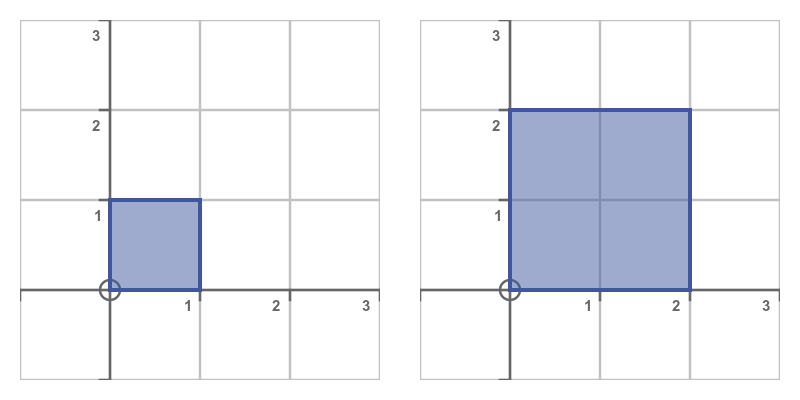
This transform scales everything out from the origin, in other words, it has the centre of enlargement of (0, 0).

Unequal scaling - stretch and squeeze transforms

This matrix scales a shape unequally in the x and y directions:

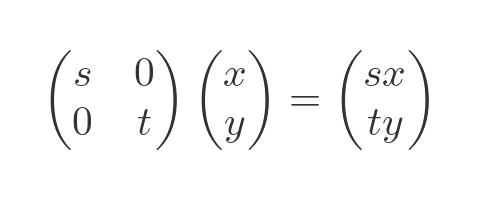
It will scale the shape by s in the x direction, and t in the y direction.

A stretch transform scales the shape along a single dimension. It is a special case of the unequal scaling above, where one of the scale factors is 1. Here is the matrix transformation to stretch in the x direction:

Here is the result for s = 2. The square is stretched by a factor of 2 in the x direction only:

A stretch in the y-direction could be achieved by swapping the 1 and s in the previous matrix.

A squeeze transform is another special case that scales the shape by s in one dimension, and by 1/s in the other dimension. Here is the squeeze matrix:

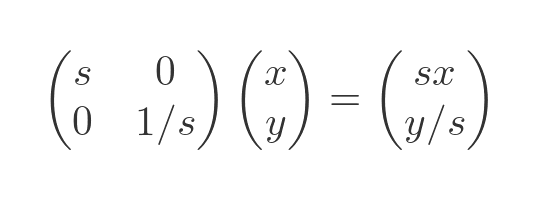
Here is the effect:

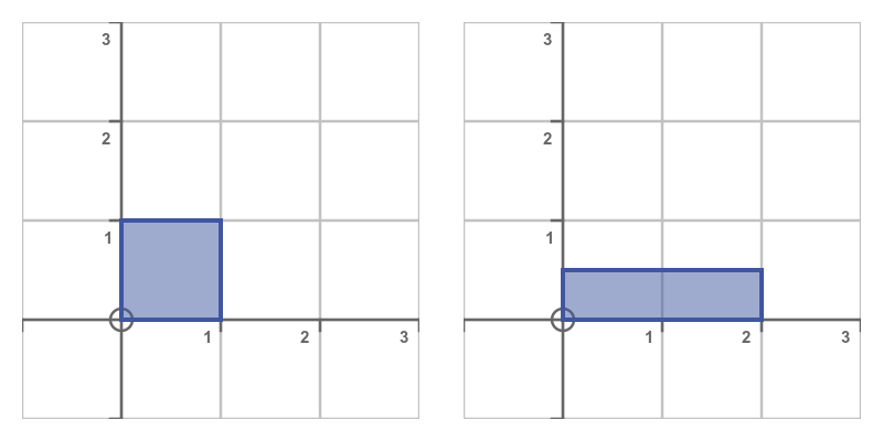
A squeeze transformation preserves area. When a squeeze matrix is applied, the width is multiplied by s and height by 1/s so the area of the shape is unchanged.

Determinants and change of area

The determinant of a matrix is a single number calculated from all the elements of a matrix. It has an important application when we look at matrix transformations:

When we transform a shape using some matrix M, then the area of the shape is multiplied by the determinant of M.

For example, the previous scaling matrix S has a determinant of:

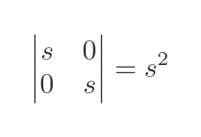
This means we would expect the matrix to scale an area by a factor of s squared. When s = 2, we would expect the area to be scaled by a factor of 4. In the earlier example, we applied the transform to a square of side 1. The result was a square of side 2, which means the area increased by a factor of 4, as expected.

In general:

• If |M| > 1 the transform enlarges areas
• If |M| < 1 the transform shrinks areas
• If |M| = 1 the transform preserves areas unchanged
• If |M| < 0 the transform includes a reflection

The identity matrix is the identity transform

We met the identity matrix in the introduction to matrices article. It is a square matrix that is all zeros, except that every element on the leading diagonal is 1. For a 2 ⨯ 2 matrix, the identity matrix is:

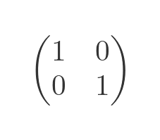
One way to think of the identity matrix is as a scaling matrix with a scale factor of 1. Of course, if we apply a scale factor of 1, it has no effect. In other words, the identity matrix represents the identity transform, i.e., a transform that has no effect.

Rotation

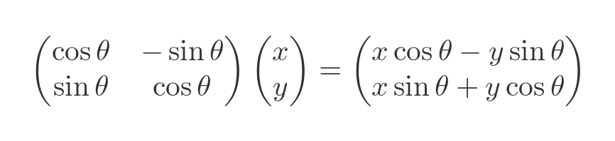
A rotation transformation uses the following matrix:

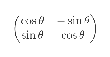
Here is the effect it has on a vector:

This rotates the shape by an angle of θ (30 degrees in this case). The angle θ is measured in radians, counterclockwise from the positive x-axis. This is the standard mathematical convention:

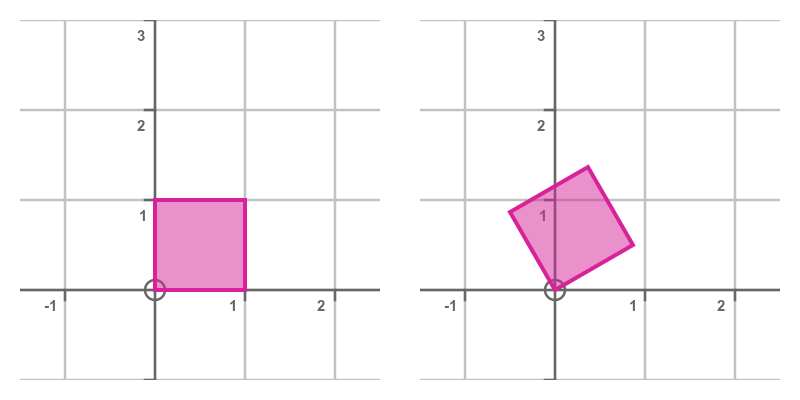
This transform rotates the shape counterclockwise about the origin. That is, it has its centre of rotation at (0, 0). To rotate clockwise, we use a negative angle, of course.

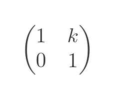
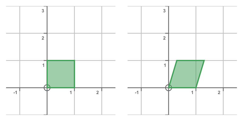
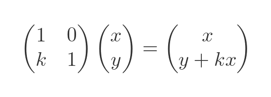
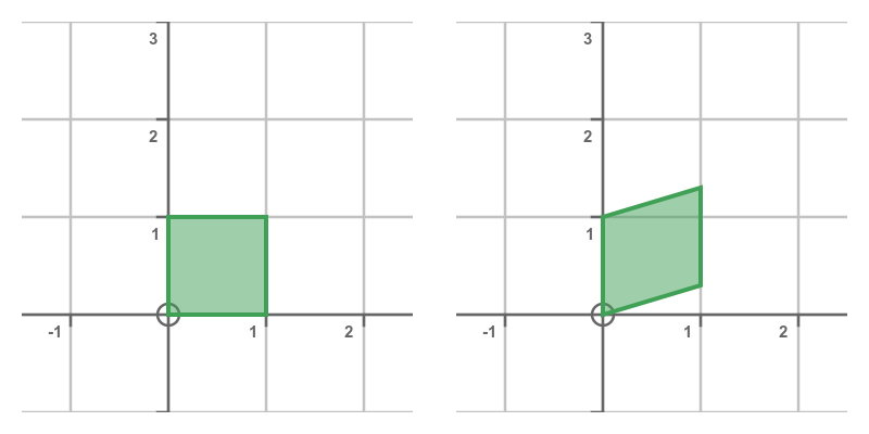
Shearing

A shear transformation slants the shape. This matrix shears horizontally:

Here is the effect it has on a vector:

This has the effect of shearing the shape:

It is also possible to shear a shape vertically, using this matrix:

Here is the result:

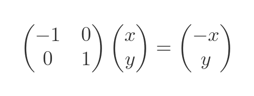
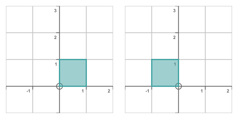
Mirroring

Mirroring a shape across the y-axis can be thought of as being a bit like stretching it in the x-direction, but with a stretch factor of -1:

Here is the result:

It is possible to mirror across the x-axis similarly, using the matrix obtained by replacing the top-left 1 with −1 and restoring the bottom-right entry to 1:

Translation

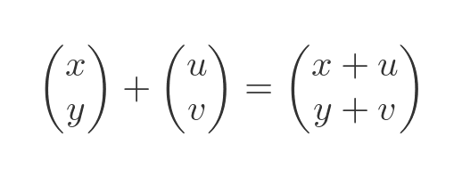
Translating a shape means moving it to a different position without changing its size, shape, or orientation. This diagram illustrates a translation by (1, 2). The square moves by 1 unit in the x-direction and 2 units in the y-direction:

We can represent this by adding 2 vectors, the original position (x, y) and a displacement vector (u, v):

But this isn't ideal. In all the other cases, we used matrix multiplication to represent the transform. It is a bit inconvenient to have to use a different calculation for translation. And in this article, we see that we can combine multiple transforms into a single matrix. To do that, we need a consistent way to represent all transformations.

To handle translation consistently with other transformations, we use homogeneous coordinates. In this system, a 2D point is represented as a 3-element vector. We create this vector by adding an extra element to the end, which always has the value 1. So the position (x,y) is represented by the vector (x, y, 1) in homogeneous coordinates.

All 2×2 transformation matrices are similarly extended to 3×3 form. This unified representation means that any affine transformation, including translation, can be expressed as a single matrix multiplication. We extend our transformation matrix by adding an extra column to the right, containing the transformation values u and v. To keep the matrix square, we also add an extra row that always contains 0, 0, 1:

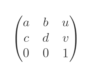
For a translation formula, we set the a, b, c, d values to a unit matrix, and set the u, v elements to contain the translation values. When we apply this matrix to a position vector, we do indeed get a translation:

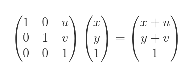
You can verify this by performing a matrix multiplication by hand (or you could use an online matrix calculator) if you wish. The third element of the transformed vector is always 1 and is discarded after the calculation, leaving us with a 2-vector result.

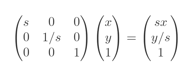
The useful thing about this is that it works for the other transformations, too. Let's try it with the squeeze transformation from before. This time we set u and v to 0 because there is no translation:

This form works for all transformations, and in this article, we see how it allows us to combine several transformations into one matrix.

Inverse transforms

Most transforms have inverses. If we apply a transform followed by its inverse, then there is no net change.

For example, scaling by 2 and scaling by 1/2 are inverse transforms. If we scale a shape by 2 and then scale the result by 1/2, we return to the original shape.

We can find the inverse of a transform by taking the inverse of the transform matrix, as explained here.

Related articles

• What is a matrix?
• Determinants
• Matrix inverse
• Combining and inverting transform matrices
• Solving simultaneous equations with matrices
• Introduction to eigenvectors
• Diagonalising matrices
• Square root of 2 by 2 matrix using Cayley–Hamilton theorem