Binary numbers

We tend to think of binary numbers as being a modern concept developed as part of computer science. But in fact, some elements of the binary system were known in ancient times, because they were very useful in many fields back then.

This article explains how binary numbers work, but it will also cover some of the history, as it is useful to know where the ideas of binary numbers came from.

Number bases - base 10

Binary numbers are simply numbers that are expressed in base 2, but before we get on to the special properties of binary numbers we will quickly look at number bases in general, starting with base 10.

You may be familiar with number bases, but even if you are not, you will certainly be familiar with base 10 (also called the denary system). Base 10 is just the way normal numbers work.

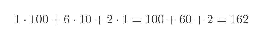
In the base 10 system, the least significant digit represents ones, the next digit represents tens, the next represents hundreds, and so on. The value of each column goes up by a factor of 10 as we move to the left, so each column is a power of 10. So, for example, the value 162 represents 1 hundreds, 6 tens, and 2 units:

The base 10 value is calculated like this:

Base 5

We don't have to use base 10, we can use any integer (greater than 1) as a base. As a second example, we will look at base 5 numbers.

In the case of base 5, the least significant digit represents 1's, the next digit represents 5's, the next represents 25's, and so on. These values are powers of 5.

To represent the number 162 (base 10) we need an extra column, which represents the value 125 (which is 5 cubed).

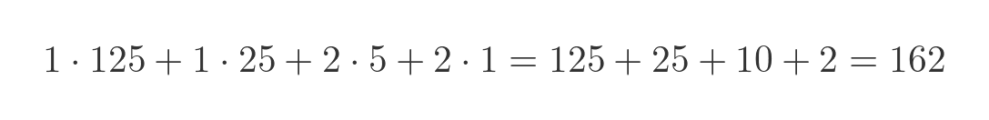
The value 162 represents is made up as follows:

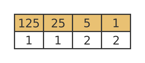
This is written and 1122₅. The base 5 value is calculated like this:

Here are the numbers 0 to 10 in base 5. The third calumn, Dec, shows the base 10 value:

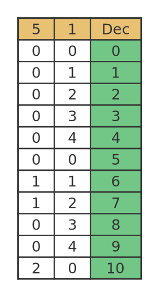
So for example, 7 is made up of 1 times 5 plus 2 times 1. 10 is made up of 2 times 5.

Notice that the least significant digit counts from 0 to 4, then jumps back to 0. Each time it resets to 0, the next digit increases by 1

Base 2

The binary system uses base 2. This means that the least significant digit represents 1', next represents 2's, then 4's, 8's, 16's and so on. These values go up in powers of 2 - in other words, each column doubles as we move to the left. The value 162 is represented like this:

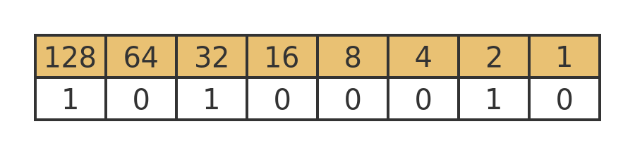
The base 2 value is calculated like this:

Base 10 uses the digits 0 to 9, base 5 uses the digits 0 to 4. Base 2 is quite special because it only uses two digits, 0 and 1. This makes it very useful because a digit can be represented by a non-numerical value such as on/off, true/false, or even the presence or absence of an object.

Here are the numbers 0 to 10 in base 2:

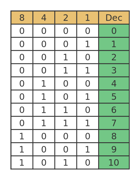
So for example, 7 is made up of 1 times 4 plus 1 times 2 plus 1 times 1. 10 is made up of 1 times 8 plus 1 times 2.

Notice that the least significant digit alternates between 0 and 1. The next digit follows a repeating pattern of 0, 0, 1, 1. The next digit repeats 0, 0, 0, 0, 1, 1, 1, 1, and so on.

Binary in ancient times - weighing scales

As we noted earlier, the binary number system was used, to some extent, in ancient times. As an example of how binary counting can arise naturally as a solution to a simple problem, we will look at weighing scales.

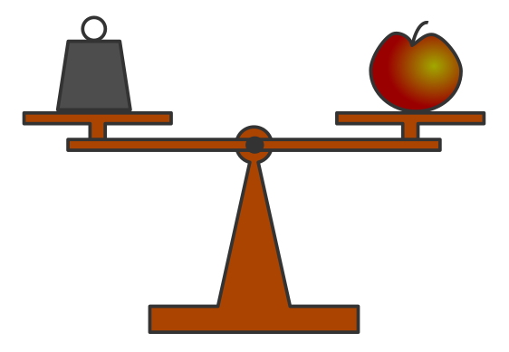
A traditional mechanical weighing scale has 2 pans. If we place an object in each pan the scale will balance if the objects have equal weight.

By placing a standard, known weight in one pan, we can add ingredients (such as flour) to the other pan, and when the scale balances we will know that we have the right amount of the ingredient:

Weighing scales of this type usually have a set of standard weights that can be used to weigh different amounts of ingredients. Prior to the widespread adoption of the metric system, many Western countries used ounces (shortened to oz) for weight. 1oz is about 25g in metric measures. We will use ounces in this description.

If we want to weigh out 1oz of an ingredient, we must place a 1oz weight on one side of the scale, and add our ingredient to the other side so that it balances. If we want to weigh 2oz, we use a 2oz weight.

But if we want to weigh 3oz, we don't need a 3oz weight. Most sets of weights don't have a 3oz weight, Instead, we take a 1oz and a 2oz weight and put them both on the scale together. Their total weight is 3oz.

To weigh 4oz we use a 4oz weight - most sets have one. By adding 1oz, 2oz or 3oz as before, we can weigh 5oz, 6oz or 7oz.

The next specific weight in the set is usually 8oz. We can use that with the other 3 weights to create every weight up to 15oz. The set may also contain a 16oz weight to allow larger weights.

The weight combination is a binary number

This list shows the weight combinations to measure weights up to 10oz:

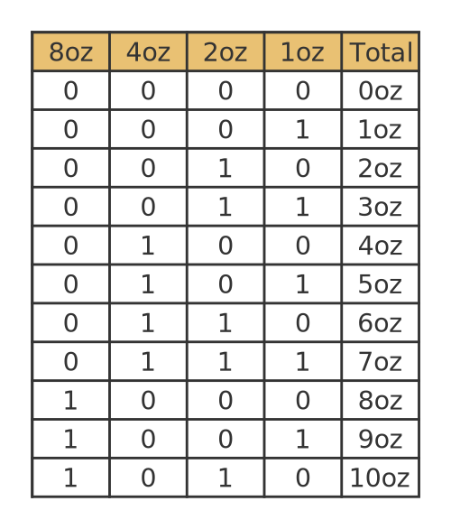
This table is identical to the binary table from earlier. The correct combination is given by a binary number, where the binary place values represent one of the weights. A one in that place indicates that the weight should be included, and a zero indicates that it should not be included. So for example to create a weight of 9oz, the binary number 1001 in the table indicates that we should use an 8oz weight and a 1oz weight.

Binary systems before computers

The mathematician Gottfried Leibniz developed some ideas on binary numbers in the 17th century. George Boole created the foundations of binary numbers and binary logic in the 19th century. The term boolean is derived from his name. For example, in mathematics, binary logic is called boolean algebra.

Systems based entirely on ones and zeros were used to store information in mechanical devices, long before electronic computers were invented. For example, the Jacquard machine used punched paper cards to control a loom to create complex lace patterns. It was entirely mechanical and was patented in the early 19th century.

In the early 20th century, electro-mechanical machines were developed that could accept data on punched cards (for example where each card contained data about an individual person) and automatically count the number of cards that met certain criteria (sex, age, etc.). These devices were precursors to computer databases and firmly established the idea of using binary representations of data.

Punched cards remained one of the main ways of transferring data into a computer right up until the mid-1970s.

Separately, electrical telegraphy was developed in the early 19th century. This allowed electrical signals to be sent long distances over wires, but in the early days technology didn't allow voice transmission, it was limited to an on/off signal. Morse code is a binary system that allows text to be sent over a single wire by encoding each character as a unique sequence of short and long pulses (effectively, zeroes and ones). This idea wasn't completely new, of course, similar systems to transmit information via drum beats or other signals go back to ancient times.

Electronic computers

When the early electronic computers were developed, first using thermionic valves and later using transistors, information was represented using voltage levels. It was possible, in principle, to use different voltages to represent different values. For example, a wire could have a voltage where 0 volts represented 0, 1 volt represented 1, right up to 9 volts representing 9. Although some systems like this were tried, as well as fully analogue computers where the voltage could vary continuously, ultimately binary processing was adopted.

In a binary electronic computer, zero is represented by 0 volts, and one is represented by the highest voltage (which is typically about 3 volts but that depends on the system). A valid signal will always be close to one of those 2 values, and never anywhere in between.

This was partly because of the legacy of binary systems that already existed, but also for practical reasons. Binary data can be manipulated by simple logic gates that can be constructed using just a few transistors each. Also, binary data is more resistant to errors - the signal is either on or off, and any small amount of electrical noise is unlikely to affect that.

Trying to process non-binary data is much more difficult than processing binary data. A binary value can be stored in a simple flip-flop circuit made from a few transistors. Storing a voltage that varies between 0 and 9 volts is a lot more difficult. Adding two binary values can be performed by a few logic gates. Adding two varying voltages, to create the correct output voltage and also a carry value if the result is greater than 9, is far more complex.

Bytes

Representing numbers, letters etc. in binary requires a combination of several single-bit values (individual 0 or 1 values) joined together to create a single value. This was clear even at the time of Morse code.

These days we use the byte as the fundamental unit of data. It is composed of 8 bits, using place values as described earlier, so it can represent an integer value between 0 and 255 (which can also be interpreted in other ways, for example as an ASCII character). Most computer processors and memory treat the byte as the basic unit of information (although they physically usually read and write multiple bytes per operation). Most network and storage systems do the same.

It wasn't always that way. In the 1950s and 1960s when electronic computing started to take off, different systems had different byte sizes, for example, 6 bits or 9 bits. The first microprocessors (integrated circuits rather than discrete logic) used a byte size of 4 bits, mainly due to technical limitations when the first chips were manufactured.

A byte size of 8 bits eventually became the standard. It is logical to have a byte size that is a power of 2 since we are dealing with binary systems. A 4-bit byte size is too small to be efficient, and 16 bits at the time would have been too large to be technically feasible, so 8 bits was the happy medium. These days most computers process 64 bits or more internally, but conceptually memory is still seen as a collection of 8-bit bytes.

Hexadecimal

A byte value looks something like this 10100011. It can be difficult to read, and also quite difficult to say. We can make it easier by using hexadecimal notation.

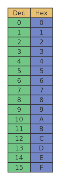
Hexadecimal numbers use base 16. This means that each digit in a hexadecimal number can take a value between 0 and 15. Of course, we only have 10 numerical characters (0 to 9), so how can we represent a number in base 16? Well, we simply use the letters A to F to represent values 10 to 15. Here is a table that maps the base 10 (dec) values 0 to 15 onto hexadecimal (hex) values:

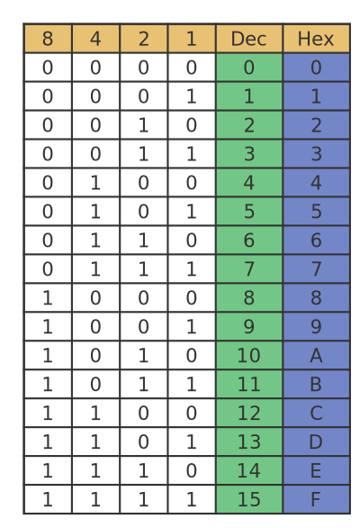
We use base 16 because a 4-bit binary value has 16 possible values. This means that a 4-bit binary quantity corresponds exactly to a single hexadecimal digit:

So the value 10100011 can be split into two 4-bit binary values 1010 and 0011. These can be represented by the hexadecimal values A and 3.

(A 4-bit binary value is sometimes called a nibble. It is like a byte only smaller.)

This means that 10100011 binary can be written and A3 hexadecimal, which is much easier to read (and say).

This becomes even more useful for larger numbers. The 16-bit binary number 0010111011010111 can be split into 0010 1110 1101 0111. In hexadecimal this is 2, E, D, 7. So the number in hex is 2ED7.

See also

• Binary addition, subtraction and negative numbers