Laplace transforms of some simple functions

We previously looked at Laplace transforms. In this article, we will look at the Laplace transforms of some simple functions (including how the transform is derived):

• The constant function, f(t) = 1.
• The exponential function.
• t to the power n, where n is a natural number.
• The Heaviside function (a step change function).
• The Dirac delta function (an impulse function).

Finding the Laplace transform of 1

The formula for the Laplace transform, as we saw in the earlier article, is:

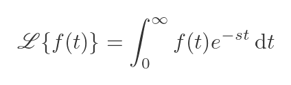
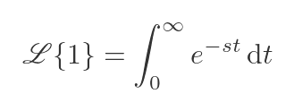
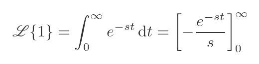
The Laplace transform operates on a function f(t) and transforms it into a different function of a different variable, F(s). In the case where f(t) is simply 1, the transform reduces to the following integral:

The integral of the exponential function is a standard result that can be found in any table of standard integrals. It is:

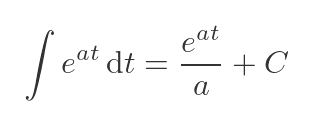
For the Laplace transform, we need to use the value -s for the parameter a, and we need to integrate between 0 and infinity.

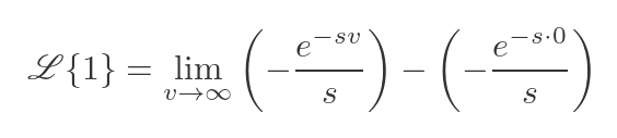
Notice that this is an improper integral, because one of the limits is infinite. We can't evaluate the integral "at" infinity, instead we must find the limit of the expression as the variable of integration tends to infinity. The first term on the RHS below represents the limit at infinity, using the limit variable v:

If we assume that s is greater than 0 (see below), then the term inside the limit gets closer to 0 as v gets larger, so the limit is 0. In the second term, t is 0, so the exponential term is 1, so the overall term is 1/s. This gives the following result for the Laplace transform:

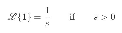
As we noted above, this transform is only valid if s > 0, because otherwise the integral will not converge (it will become infinite as t approaches infinity). When we use the Laplace transform, we normally do a calculation in s space, and then convert back to t space. In most cases, we don't need to worry about the values of s. We will cover some cases where we need to take the value of s into account in a later article.

Laplace transform of exponential function

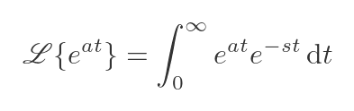
Next, we will look at the Laplace transform of the exponential function. We will use an exponent of at (where a is a constant). We substitute this function for f(t) in the standard formula:

We are multiplying two exponentials, so we can simplify the expression by adding the exponents:

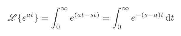
Now we could solve this in a similar way to the previous example, and you are welcome to do that as an exercise if you wish. But we will take a shortcut here. We have deliberately expressed the exponent as a negative expression, because that makes it look similar to the previous example. In fact, it is identical to the previous example except that the s has been replaced by s - a. So we can use that substitution to solve the integral directly:

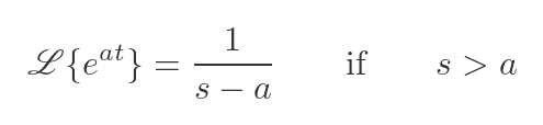
We have just replaced s with s - a in the previous case. Notice that this means that s must be greater than a, rather than 0, in the previous example.

Laplace transform of t to the power n

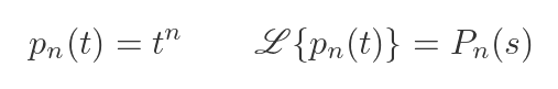
As another example, we will find the Laplace transform of tⁿ. But we will do that in a slightly different way to the previous cases. We will use differentiation and induction. It will make things easier if we define a function p_n to represent t to the power n, and its Laplace transform, P_n:

Our approach will be to find the Laplace transform of the derivative of p_n. There are two different ways to do this, and combining the two methods gives a relationship between P for n and P for (n - 1) that we can use to perform induction.

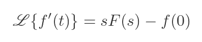
For the first method, there is a general Laplace transform for f'(t), for any f(t). We derived this in an earlier article. The general formula is:

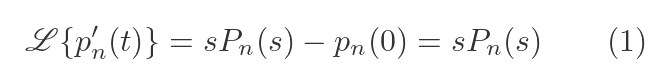
We can apply this specifically to p. Since p_n(t) is tⁿ, it follows that p_n(0) is 0ⁿ, which of course is 0. So that term can be removed. This leaves the following:

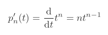
There is a second way to find the Laplace transform of p'. We can first differentiate p. This is just the derivative of tⁿ:

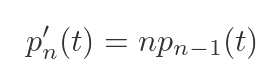
But, of course, t to the power (n - 1) can also be expressed as a p function:

We then take the Laplace transform of both sides. Since n is a constant, we can move it outside the transform (as we proved we could do in the previous article):

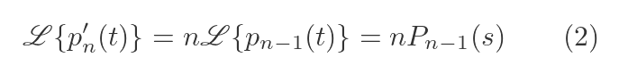
Equations (1) and (2) both give the Laplace transform of p', expressed in different ways. We can therefore equate the RHS of both equations:

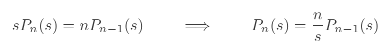
This gives us an expression for Laplace transform n in terms of transform n - 1. So if we know the transform for n - 1, we can find the transform for n

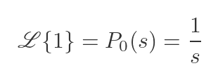
And we do know the transform for n is 0. p₀(t) is t⁰, which is 1. We found the Laplace transform of 1 earlier, so we have::

When n is 1, t to the power 1 is t, so we can find the Laplace transform of t:

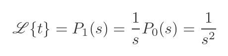
If you read the previous article, we found this transform using a different method, but of course, the result was the same.

To find the transform of t squared, we multiply the transform of t by 2/s:

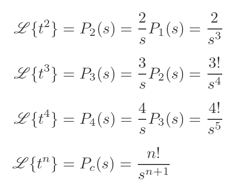
Some other results are shown above. To find the transform of t cubed, we multiply the transform of t squared by 3/s. The numerator becomes 3 times 2 (times 1, not shown), which is 3 factorial, and the denominator becomes s to the power 4.

The result for t to the power 4 is also shown. The pattern should be clear at this point, the Laplace transform for t to the n is n factorial divided by s to the power n + 1.

Heaviside step function

Laplace transforms are often used practically for solving differential equations in physical systems. One example is analysing the behaviour of electronic circuits.

Step functions are often useful in this context. For example, when an electronic system is first switched on, the supply voltage goes from 0 to whatever voltage the circuit operates at, some voltage V. For simplicity, we often model that as a step function that is initially 0 but instantly changes to V when the switch is flipped.

The Heaviside step function is a function that is defined to have a value 0 for t < 0, and a value of 1 for t >= 0. We will write the as u(t) (it is also sometimes written as H(t), but that clashes with our notation of using uppercase letters for transformed functions). Here is a graph of the function:

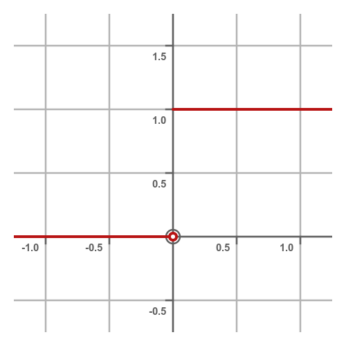
As the graph shows, the value is 0 for negative t and 1 for positive t, with a discontinuity (a step change) at 0. The value is 1 when t is 0. The small circle at the origin indicates that the negative line doesn't extend to 0.

What is the Laplace transform of u? We can use the normal Laplace equation to find this:

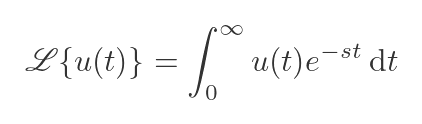
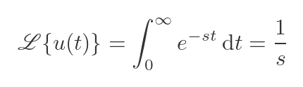
But, of course, the integral is over the range 0 to infinity, and over that range u is equal to 1. So the Laplace transform of the Heaviside function looks identical to the Laplace transform of 1, which we calculated earlier:

It is also useful to calculate the Laplace transform of u(t - a), where a is some positive constant. This function is similar to the normal Heaviside function, except that the transition from 0 to 1 happens when t equals a:

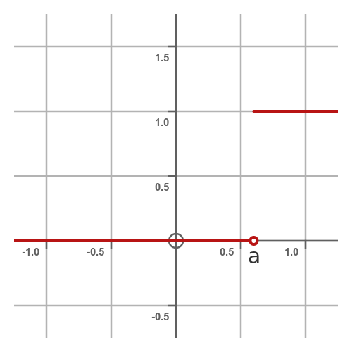
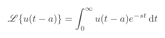
In the example of an electronic circuit, this might represent a switch being activated while the circuit is already operating. We can find the Laplace transform of this function by substituting t with t - a in the earlier equation:

There is an easy way to simplify this integral. Remember that u(t - a) is 0 when t < a. This means that the entire expression under the integral sign is 0 when t < a. So we only need to calculate the integral from a to infinity.

Remember, too, that u is 1 when t >= a. So we can discard the u term from the integral. Making those two changes, our integral now becomes:

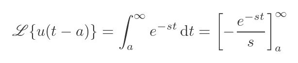
This is just like the Laplace transform of 1, except the range starts at a rather than 0. We evaluate it in the same way:

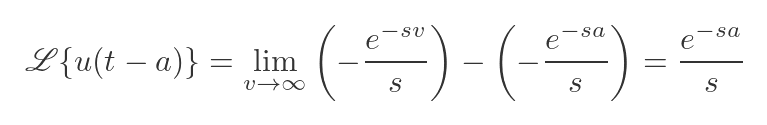
Once again, the first term goes to 0 as v tends to infinity, so we are left with just the second term.

The Dirac delta function

Sometimes we need to model impulses in physical systems. An example of that might be hitting a golf ball with a club. When the club hits the ball, it imparts a finite amount of energy to the ball, but in a very short time. We often approximate that by saying that the impact is instantaneous, that is, it takes zero time. The ball starts at rest, but at the moment it is hit, it immediately starts travelling at some velocity v.

Since its velocity changes from 0 to v in zero time, its acceleration at the moment is infinite. You might normally expect that, if we apply infinite acceleration to an object, the object would gain infinite velocity. But in this case we are applying infinite acceleration for zero time. Infinity multiplied by zero is indeterminate. We need to use limits to determine the outcome.

Suppose we applied an acceleration of 1 ms^-2 for 1 second. The resulting velocity would be 1 ms^-1. This is the magenta curve on the graph below. The curve shows acceleration against time, the final velocity is the area under the curve:

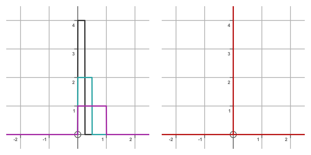
If instead we apply an acceleration of 2 ms^-2, but for only for 0.5 seconds (cyan curve), the area under the curve is still 1, so the velocity is 1. If we apply an acceleration of 4 ms^-2 for 0.25 seconds (black curve), again, the area and final velocity are 1.

If we continue halving the width and doubling the height of the curve, the area under the curve and, therefore, the resulting velocity of the ball, will always be 1. In the limit, the curve will tend towards a rectangle of infinite height, zero width, but still containing an area of 1. This is shown in the RHS graph, above.

The limiting function is called the Dirac delta function, written as δ(t). It is a pulse of infinite height, zero width, but with an area of 1.

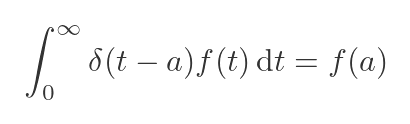
One property of the Dirac delta function, which we won't prove here, is the following:

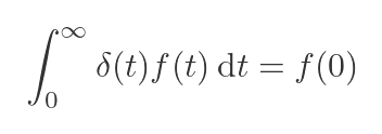
The integral of δ(t) multiplied by some function f(t) is equal to f(0). Why is that? Well, we know that the area under δ(t) is 1. But we also know that δ(t) is 0 for any non-zero value of t. At t = 0, δ(t) has an area of 1, but it is multiplied by the value of f at that point, which, of course, is f(0). So the area under the function δ(t) times f(t) is just f(0).

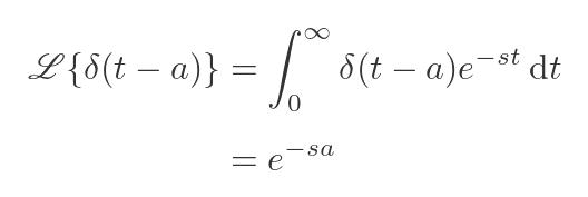
What is the Laplace transform of the delta function? We just apply the standard Laplace definition to δ(t):

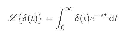
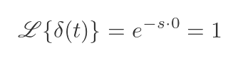
This looks very much like the previous equation, using the exponential in s for the function f(t). As we know, this integral evaluates to f(0), which in this case is simply 1:

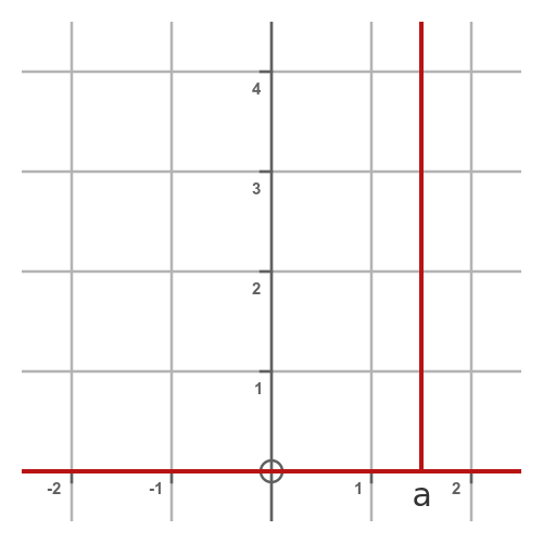
What about an impulse that happens at some other time, for example, at time a (where a is positive)? Similar to the Heaviside function case, we can write this as δ(t - a). Here is the graph:

This time, the integral of δ(t - a) multiplied by some function f is equal to f(a) (rather than f(0)):

For the Laplace transform, this gives a result of:

Related articles

• Introduction to Laplace transforms