Combining and inverting transform matrices

We previously looked at using matrices to represent transformations in 2 dimensions. As we will see here, we can apply compound transformations (such as scale and rotate) by applying several matrices. We can also calculate the inverse of a transform simply by inverting the matrix.

This in turn allows us to switch between different frames of reference to define transformations, for example, to allow us to rotate a shape about its own centre. We can also use matrix algebra to represent a combination of transformations as a single matrix, which means the transformations can be applied very efficiently.

Using 3 by 3 matrices

In the earlier article on transformations, we introduced the idea of using a 3 by 3 matrix, which allows us to represent translation via matrix multiplication:

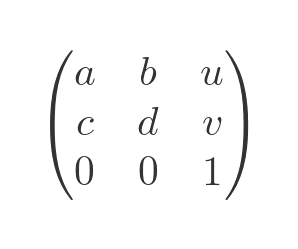
The values a to d represent the values in a normal 2 by 2 matrix, u and v represent the x and y translation, and the bottom row is always (0, 0, 1).

This matrix needs a 3-vector to operate on. This is formed by adding an extra element, which is always 1, to the normal (x, y) vector:

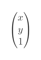
In this article, since we are dealing with general, combined, transform matrices, we will always use the 3 by 3 form, even when u and v happen to be 0.

Scaling and rotation transformations

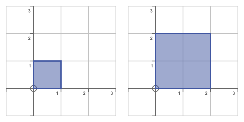
Here is a simple scaling transformation. We looked at this in the previous article. It scales the shape by a factor of 2:

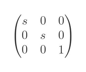
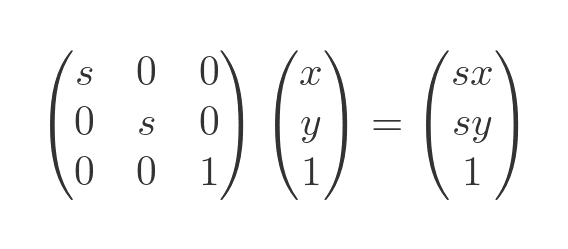
This is the scaling matrix. Again we looked at this in the previous article, but this time we have expressed it as a 3 by 3 matrix:

This is the result of applying the scaling matrix to a vector (x, y). Notice that the resulting vector still has a 1 and its third element, which we ignore when looking at the 2-dimensional result:

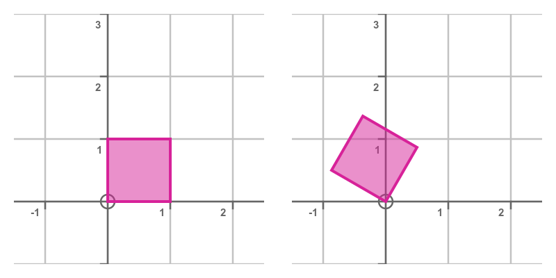
Here is a simple rotation transformation. It rotates through an angle θ, counterclockwise. In this case, θ is 60°:

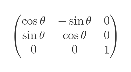
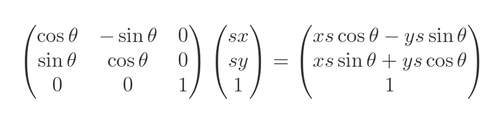
This is the rotation matrix:

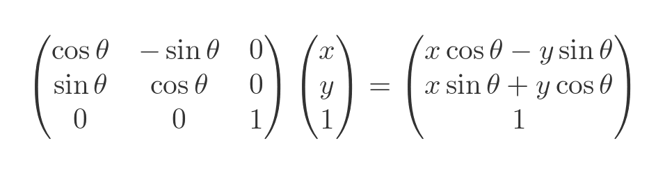
This is the result of applying the rotation matrix to a vector (x, y):

Combining the two transformations

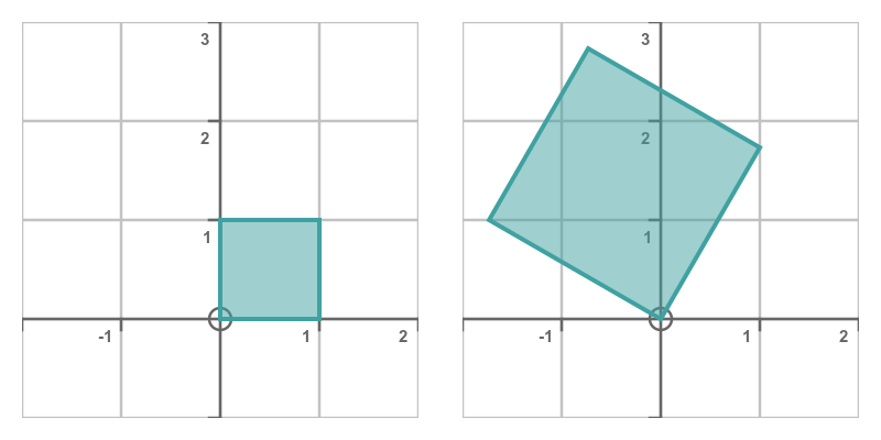
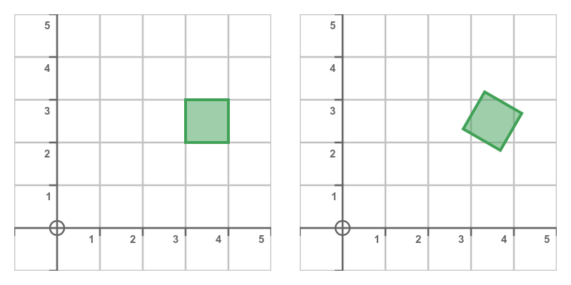
If we scale and rotate the shape, we get this:

One way to calculate this is to first scale the vector, and then rotate it. We already know the scaled vector:

If we apply the rotation matrix to this scaled vector we get the rotated, scaled vector:

This is a perfectly valid way to calculate the transformation, but it is possible to reduce this to a single matrix multiplication, and this can often have advantages as we will see below.

To start with, we can write this process symbolically:

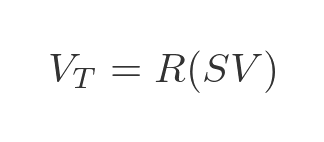
Here V is the original vector, S is the scaling matrix, and R is the rotation matrix. We have calculated the transformed vector VT using matrix multiplication in the order implied by the brackets.

But remember that matrix multiplication is associative - that is to say, we can perform the multiplications in any order. So we can do this:

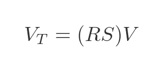
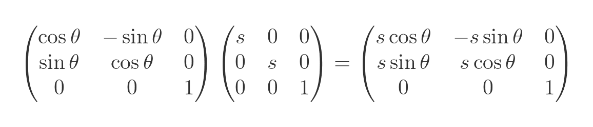
This means that we can first multiply the transformation matrices together to obtain a combined matrix that applies both transformations in one step:

Why does this matter? Well in some applications, such as computer graphics, we might want to apply the same transformation to many thousands of points. For animated graphics (such as games) we might want to do that many times per second. Using the first method, we must perform two matrix multiplications on each point. Using the second method we just need to calculate the compound matrix once, and then we only have to perform one matrix multiplication on each point.

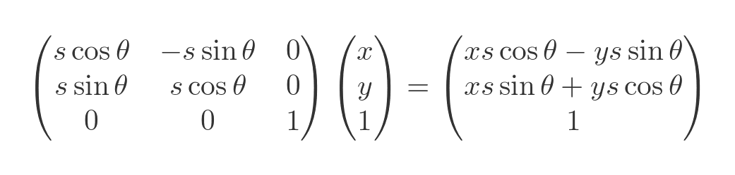
Here is the result of multiplying the original vector by the compound matrix, to verify that it gives the same result as before:

Inverting a transform

The inverse of a transform has the opposite effect of the transform. Put another way, the inverse of a transform undoes the effect of that transform.

For simple transforms, we can easily work out the inverse matrix. For example, we saw earlier that this matrix scales by a factor s:

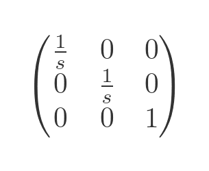
If we have scaled a shape by a factor of s, what do we need to do to undo that scaling? Well of course, we need to scale it again by a factor of 1/s and the resulting shape will be back to its original size. The matrix for scaling by a factor of 1/s can be found by simply substituting 1/s for s in the previous scaling matrix:

As another example, take the rotation matrix from before:

This transform rotates the shape by angle θ, counterclockwise. How do we undo such a transform? We simply need to rotate clockwise by θ, or (equivalently) we need to rotate counterclockwise by -θ:

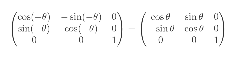
The matrix on the right has been simplified using the symmetric properties on the sine and cosine of a negative angle - sine of minus theta equals minus sine theta, and cosine of minus theta equals cosine theta.

The inverse transform is the inverse matrix

From the discussion above, if we apply a transform matrix A, followed by its inverse transform B, then B undoes the effect of A. So we can say that the net effect of the product of these two matrices is to leave the shape unchanged. This means that BA must equal the unit matrix, since any other matrix would alter the shape in some way:

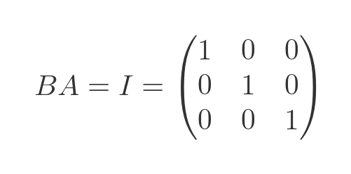
This in turn means that B must be the inverse matrix of A

This is quite a nice result. Firstly it shows that a matrix is a very natural way to represent a transform. Secondly, from a practical point of view, it gives us a process to find the inverse of any reversible transform. Note that some transforms cannot be reversed, and we will see that the matrix representation gives us a way to detect that too.

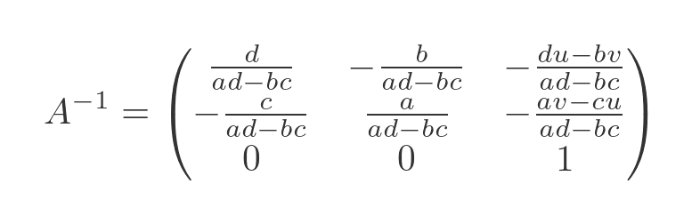
The linked article on inverse matrices shows the general formula for calculating the inverse of a matrix. However, when it comes to transform matrices remember that the matrix is somewhat simplified because the third line is always 0, 0, 1:

We can find the inverse of this matrix using the standard formula from the article mentioned above. The calculation is quite long and tedious, but not particularly complicated, so we will skip it here and jump straight to the result:

To take the example of a scaling matrix:

We have:

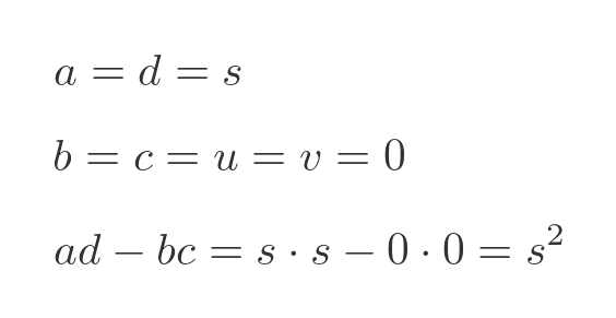
And since u and v are zero we have:

If we substitute these values into the general equation we get:

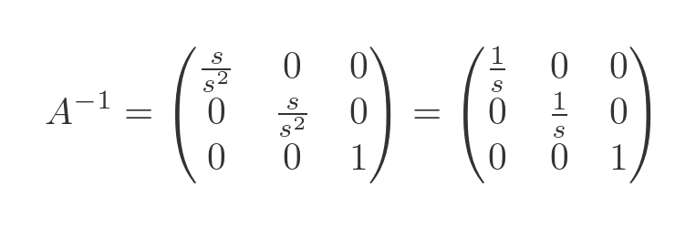
As expected, this is the same as the inverse scaling transform that we calculated earlier.

Irreversible transformations

Suppose we used the zero matrix (a matrix filled entirely with zeros) as a transform. This would map every point in space onto the origin, (0, 0). If we then attempted to reverse this transform, it wouldn't work, because every point in the transformed shape would be (0, 0) so it would be impossible to map each point back to where it came from.

This doesn't just happen for the zero transform. If we transform using any matrix that doesn't have an inverse, then we can't reverse it. In general, a transform is irreversible if its determinant is zero.

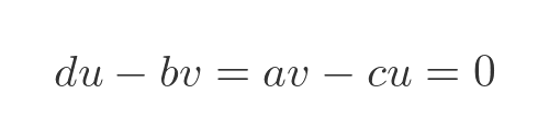
However, in the special case of a 2-dimensional transform, the determinant will be 0 if a.d equals b.c. In that case, the denominator in the inverse matrix above will be zero, so it will be impossible to calculate an inverse matrix.

Changing the frame of reference

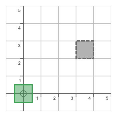
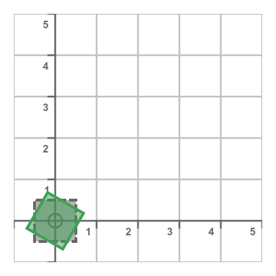
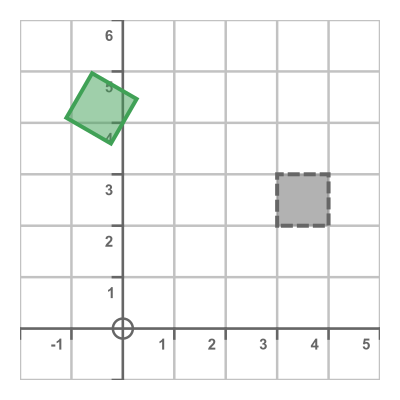
What if we wanted to rotate this shape about its centre? Like this:

How might we do that? Well, we know how to translate the original shape (in grey) so that it is centred on the origin:

Here is the transform matrix (notice that we move the shape by an extra 0.5 so that it is centred on the origin):

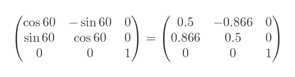
We can then rotate the shape about the origin by 60°:

Here is the transform matrix, with its approximate numerical value:

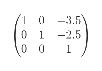
Finally, we translate the shape back so that its centre is back to its original position:

This is done by applying the inverse of the previous translation. The result is the shape rotated about its centre:

If we combine the three transforms we get a single transform that rotates the square about its centre:

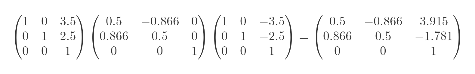
Alternative view of change of frame of reference

There is yet another way to view this transform, which is also quite interesting. The final matrix given above can be viewed as a rotation by 60° about the origin, followed by a translation by (3.915, -1.781).

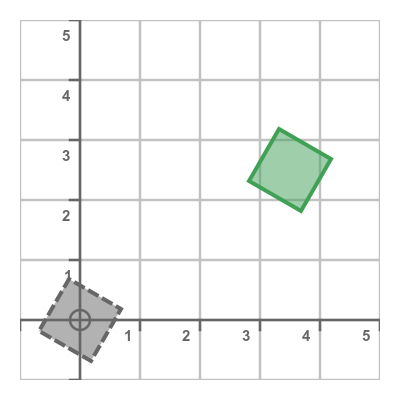
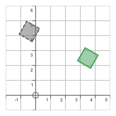
First here is the rotation. Since we are rotating about the origin, the square is rotated by 60°, but in addition, it is moved to a completely different place:

Now if we translate the square by (3.915, -1.781), then it moves back to its original position (its centre is in exactly the same place as the original square) but still rotated by 60°:

See also

• What is a matrix?
• Determinants
• Matrix inverse
• 2D transformation matrices
• Solving simultaneous equations with matrices
• Introduction to eigenvectors
• Diagonalising matrices